What is Spark shuffle?
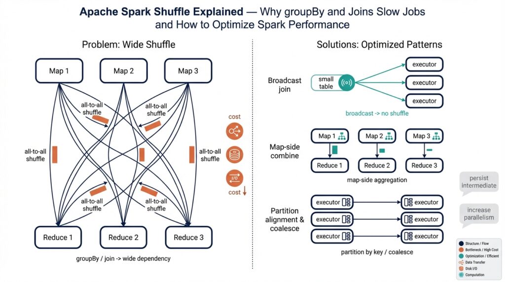
Imagine you just ran a groupBy and watched your Spark job stall — you’re not alone. Spark shuffle is the behind-the-scenes reorganization that forces that pause: shuffle (in plain language) means moving records across the cluster so that all entries with the same key end up on the same worker. In simple terms, Spark shuffle is the data-moving step Spark performs when it must regroup or redistribute data; it’s the reason many groupBy and joins suddenly become slow and chatty across the network.
First, let us meet a few characters so the story makes sense. A partition is a slice of your dataset that lives on one worker, a task is a unit of work that processes a partition, and an executor is the JVM process on a worker node that runs many tasks. When an operation requires records with the same key to co-locate (for example aggregation by key or joining two tables on a key), Spark decides it cannot do that solely inside each partition — it must reshuffle records across partitions. That movement is the shuffle: writing data out, sending it across the network, and reading it back in new places.
How does this movement happen? Picture a team of cooks making different dishes who realize each recipe needs ingredients grouped by spice type. Each cook writes their spices into labeled boxes (this is the shuffle write), a delivery van transports boxes between kitchens (network transfer), and the cooks at the destination open the boxes and use the spices together (shuffle read). Concretely, Spark performs a map-side step that writes out records grouped by destination partition, transfers those files across the cluster, then runs reduce-side tasks that read the incoming data and perform the aggregation or join.
Why does Spark shuffle slow down groupBy and joins? Because moving data is expensive. The shuffle produces disk I/O when intermediate files are written, network I/O when blocks are transferred, CPU time for serializing and deserializing records, and memory pressure that can cause spills to disk. Each of these costs multiplies with data size and cluster scale, so an innocent-looking groupBy or join can balloon into the most expensive part of a job and harm overall Spark performance.
Let’s make this concrete with a short example in your head: you have 100 partitions, and a groupBy key that’s common across many partitions. Every partition must send matching keys to the appropriate target partition, so you get up to 100× of outgoing and incoming transfers. If one key is extremely frequent (data skew), one partition becomes the bottleneck and slows every dependent task. That skew, plus repeated serialization and I/O, explains why some groupBy and joins feel painfully slow even when raw data sizes seem moderate.
Knowing what shuffle is gives you a compass for action: reduce unnecessary reshuffles, prefer map-side aggregation when possible, and watch out for skew. Building on this foundation, we can now explore concrete techniques that change how and when data is moved so you keep more work local, reduce disk and network pressure, and improve Spark performance without changing the outcomes of your computations.
When shuffles occur
Imagine you just kicked off a job that uses groupBy and joins and then watched tasks hang while network and disk lights blink furiously — that pause is a Spark shuffle at work. Spark shuffle (the cluster-level reorganization that moves records so matching keys end up together) shows up whenever Spark cannot complete a computation inside the partitions it already has. Building on what we covered earlier, this section walks through the concrete moments when that data movement starts, so you can spot, predict, and avoid expensive shuffles when possible.
First, let us introduce two characters who decide whether a shuffle is needed: narrow and wide transformations. A narrow transformation is an operation where each input partition maps to exactly one output partition — examples are map and filter — and these do not require moving data between workers. A wide transformation requires data from many input partitions to be grouped into fewer or different output partitions; wide transformations force a shuffle because Spark must physically move records across the network so related keys meet. Thinking of it like a neighborhood potluck: narrow work is cooking alone in your kitchen, wide work is gathering everyone’s dishes at a single table.
Which Spark operations are commonly the culprits that trigger wide transformations and therefore shuffles? Operations that require grouping or global reordering cause shuffles: groupByKey, groupBy (the higher-level grouping), reduceByKey and aggregateByKey (both are wide but can do partial aggregation), joins and cogroup, distinct, repartition (when you explicitly change partitioning), and sort operations that need a global order. These are the moments Spark draws a line between map-side (where tasks run independently) and reduce-side (where reorganized data is consumed) stages — the line is a shuffle boundary.
Not all wide operations are equally painful because some include helpers that reduce the cost. Map-side aggregation (also called a combiner) is a technique where Spark partially aggregates values before sending them across the network. For example, reduceByKey differs from groupByKey in that reduceByKey performs partial reductions on each partition first, so the amount of data shuffled is often much smaller. In plain terms: reduceByKey packs the suitcase before the flight; groupByKey throws everything into the cargo hold and hopes for the best.
Joins deserve special attention because they’re a frequent source of slow jobs. A regular shuffle join moves matching rows across the cluster so equal keys land together and then combines them — that’s a classic wide transformation. Spark, however, can avoid that shuffle by using a broadcast join: if one side of the join is small enough, Spark will copy (broadcast) the small dataset to every worker so the larger dataset can be scanned locally. Knowing when Spark will broadcast and when it will shuffle is essential to optimizing joins and preventing unnecessary network traffic.
Repartitioning and coalescing are another pair to understand. repartition explicitly reshuffles data to a new number of partitions and always triggers a shuffle (useful for balancing). coalesce reduces the number of partitions without a full shuffle when you allow some imbalance; it’s faster but can create skewed partitions. In short: repartition is a full neighborhood move, coalesce is folding a few houses into one without moving everything.
How do you know when a shuffle actually happened in a running job? Look at the Spark UI: shuffle write and shuffle read metrics appear per stage, and stage boundaries mark shuffle points. You can also infer shuffles by the presence of wide transformations in your code and by watching for long stages that show heavy disk or network I/O. Asking “How do you know when a shuffle will occur?” is a good habit — once you can predict it, you can plan to reduce it.
Understanding exactly when shuffles occur gives you a practical map for optimization: prefer map-side aggregation where possible, choose reduceByKey over groupByKey when you only need an aggregate, broadcast small tables for joins, and avoid unnecessary repartitioning. With these patterns in mind, you’ll reduce Spark shuffle overhead, combat data skew, and keep more work local — which is exactly the kind of leverage that turns a slow job into a fast one.
groupBy vs reduceByKey
Building on this foundation about why data movement kills performance, imagine you’re deciding how to collect values by key and you must choose between two common approaches in Spark. Spark shuffle is the invisible tax you pay when keys have to meet on the other side of the cluster, so the choice you make here directly controls how much network and disk I/O will happen. We’ll walk through the two patterns as if they were teammates with very different habits, and by the end you’ll know when to let one of them drive.
First, meet the two teammates by name and role. One operation gathers every value for a key and hands the whole bag to the downstream task; this is what people mean when they call groupByKey (or higher-level groupBy) — it literally groups all values for each key together. The other operation asks each partition to do a bit of work first and only send a smaller summary onward; reduceByKey performs a reduction (an aggregation that combines values) at the map side before the shuffle. Define a key as the thing you’re grouping by (like a word or userId) and a value as the associated payload (count, record, or metric); define a combiner as the partial aggregator that runs on each partition to shrink data before it’s moved.
The practical difference lives in how much gets packed into the network van. With groupByKey, every value for a given key from every partition is sent across the cluster and then collected on the reducer — that means potentially huge shuffle writes and reads, lots of serialization, and more disk I/O. With reduceByKey, Spark runs a map-side combine that merges values per key inside each partition, so the data that actually crosses the network is already condensed. Think of it like packing for a trip: reduceByKey folds and compresses your clothes at home, while groupByKey throws everything into separate suitcases at the airport.
Let’s make this concrete with a common example: counting words. You start with pairs like (“spark”, 1) for every occurrence. If you use groupByKey then every “1” for the same word travels to the reducer and the reducer does all the summing — that means many small values are shuffled. If you use reduceByKey Spark will sum the ones inside each partition first (making a small local count) and only those local counts are shuffled and summed again. This difference often reduces shuffle volume by orders of magnitude for large datasets and directly speeds up jobs because fewer bytes move and less disk I/O happens.
When should you pick one over the other? If you actually need the entire list of values for a key (for example, to preserve ordering or to produce a collection like a list), then groupByKey or a grouping operation is the correct tool; you can’t invent the original list from just reductions. But if your goal is an associative aggregation (sum, min, max, count, or combineable statistics), prefer reduceByKey or aggregateByKey because they perform map-side aggregation and lower shuffle pressure. Ask yourself: do I need all the raw values, or is a reduced summary sufficient? That question will guide the right choice.
There are a few practical caveats to keep in mind as we move toward optimization. Data skew can still make a reducer the hotspot even with reduceByKey if one key dominates; consider salting or pre-aggregating to spread work. For more complex value types where you need customized combine logic, aggregateByKey or combineByKey offer the same map-side combining benefits with finer control. Instrument your job with the Spark UI to check shuffle write/read sizes and stage boundaries so you can verify that you actually reduced network traffic.
Now that you understand how these two approaches differ in behavior and cost, you can choose the pattern that minimizes Spark shuffle for your workload and improves job latency. With that decision made, let’s take the next step and look at how joins and partitioning choices interact with the same map-side combining ideas we just explored.
How joins trigger shuffles
Imagine you’re joining two tables and the job suddenly grinds to a crawl: Spark shuffle is thrumming, disks are busy, and network lights blink. Spark shuffle (the process of moving records across the cluster so matching keys land together) is often the invisible reason joins become slow. In joins we must bring rows that share a join key into the same place; if Spark can’t do that locally, it reshuffles data across partitions. That tension—wanting rows to meet but having them scattered—explains why joins and Spark shuffle are so tightly linked.
First, let’s name the basic players so the scene is clear. A partition is a slice of your dataset that lives on one worker; co‑partitioned means two datasets are laid out using the same partitioning scheme so matching keys already share partitions. When keys aren’t co‑partitioned, Spark must perform a shuffle: each task writes out slices of its partition for destination partitions (shuffle write), those slices travel over the network, and tasks on the receiving side read them (shuffle read). Picture neighbors mailing ingredients to a community kitchen so everyone cooking the same recipe ends up with the same spices.
Spark chooses between a couple of join strategies and each has different shuffle behavior. A broadcast join (broadcast: copying a small dataset to every executor) avoids a cluster‑wide shuffle because the small side is available locally on every worker; Spark will do this when one side is small enough to copy. By contrast, a shuffle‑based join (commonly implemented as a sort‑merge join) redistributes both inputs by the join key so equal keys land in the same partition, then sorts and merges them to produce results. There are also in‑memory hash joins when a side fits into executor memory; those can avoid costly sorts but still may require shuffling to align keys.
To see the cost in plain terms, imagine two big tables with 100 partitions each and a join key spread across them. If neither side is broadcastable, every partition from the left may need to send rows to many partitions on the right and vice versa—this can produce many-to-many transfers and lots of disk/network I/O. If one key is extremely frequent (data skew), one receiving partition becomes the hotspot and throttles the entire join stage. That combinaton of many transfers, serialization, and skew explains the long stalls you’ve watched in the Spark UI.
So what practical options do you have to reduce shuffle pain? If one side is small, prefer a broadcast join: give Spark a hint or rely on the optimizer to broadcast the small dimension table so the large table can be scanned locally on each executor. If both datasets are large, consider pre‑partitioning them by the join key (repartitioning them with the same partitioner) so they become effectively co‑partitioned; be mindful that repartition itself triggers a shuffle, so this is worth doing when you’ll reuse the partitioning. Another technique is bucketing (physical layout that groups rows by key) which, when aligned between tables, can allow more map‑side joins without an extra reshuffle. If skew is the problem, salting (adding a small random prefix to the join key to spread hot keys across partitions, then removing the prefix after) can help distribute work.
How do you know which choice to make? Ask: When should you broadcast instead of shuffle? If one table is small enough to fit in memory on every executor, broadcast. If both tables are large, aim to ensure they are co‑partitioned or bucketed on the join key before joining, or use salting for skewed keys. Verify your choice in the Spark UI: stage boundaries, shuffle write/read sizes, and executor metrics will tell the story. With these patterns—broadcasting small sides, co‑partitioning or bucketing large ones, and mitigating skew—you control when Spark shuffle happens and reduce the join stages that dominate job time.
Building on what we learned about groupBy and reduceByKey, the next step is to look at how partition counts and executor memory settings influence whether a join becomes a map‑side miracle or a full cluster shuffle; that will show us how to tune resources so joins behave more predictably.
Detecting shuffle and data skew
Imagine you just watched a stage take forever and wondered whether the slowdown came from shuffle or data skew — those two are the usual suspects. Shuffle (the cluster-wide movement of records so matching keys meet) and data skew (when a few keys dominate your data distribution) show up as performance fingerprints you can learn to read. Building on what we covered earlier about partitioning and map-side aggregation, this section walks beside you as we look for the telltale signs in the UI, in task timings, and in simple programmatic checks so you can spot trouble before it ruins the whole run.
First, how do you know a shuffle happened and whether it’s the problem? The Spark UI is your detective board: stage boundaries indicate shuffle points, and each stage shows shuffle write/read bytes and shuffle file counts. Shuffle write is the data each map task outputs for downstream reducers; shuffle read is the data each reduce task ingests — large numbers or sudden spikes in these metrics mean a lot of bytes moved across the network. Watch for long shuffle write times, high shuffle spill-to-disk counts, and stages where many tasks finish quickly except a handful that run much longer; those are the first clues.
Now let us look for signs of data skew specifically. Data skew (an uneven distribution of keys so some partitions get far more records) usually appears as a small number of tasks taking disproportionately longer and processing far more bytes or records than the rest. In the Spark UI you’ll see a tailed task duration chart: most tasks finish quickly, while one or two stragglers chew time and resources. You can also spot skew by comparing “Input Size / Records Read” across tasks in a stage — a huge variance is a red flag that a few partitions hold most of the work.
We don’t have to rely only on the UI; you can run quick programmatic checks to confirm skew. A low-cost technique is sampling partition sizes: run something like rdd.sample(false, 0.01).mapPartitions(iter => Iterator(iter.size)).collect() to get a rough distribution without scanning everything. If you need exact counts, rdd.mapPartitions(iter => Iterator(iter.size)).collect() will tell you how many records live in each partition, but beware this touches all data and can be expensive. For joins, inspect the small/large side sizes: if one join key consistently maps to huge local counts or one partition’s shuffle read is orders of magnitude larger, that’s practical evidence of skew.
There are a few other runtime signals worth checking before you start refactoring code. Look at executor-level metrics: high garbage-collection time or repeated spill events on one executor often accompany skewed partitions. If you use the SQL tab, check job descriptions that list shuffle read/write sizes and check the Job DAG — stages with massive shuffle read/write sizes are the hotspots. For long-running or production systems, consider adding a lightweight Spark listener that records per-task input sizes and durations so you can track skew trends over time rather than chasing a single failed run.
Detecting shuffle and data skew gives you the power to target fixes instead of guessing. When you’ve confirmed a shuffle is heavy or a key is skewed, you’ll know whether to try pre-aggregation, salting the hot key, increasing parallelism for the affected stage, or using a broadcast join for a small side — tactics we introduced earlier. With these detective skills, you move from reacting to shuffle surprises toward making deliberate, evidence-based changes; next, we’ll use that information to tune partition counts and memory so your job spends less time moving data and more time doing useful work.
Practical shuffle optimization techniques
Imagine you’ve already seen a stage stall because of Spark shuffle and you want practical levers to stop the bleeding. Spark shuffle — the cluster work that moves keys so matching records meet — is the expensive operation we’ll learn to avoid or shrink. In the next few paragraphs we’ll treat each optimization like a tool in a chef’s kit: when to reach for it, how to use it, and what trade-offs to expect so you can make informed changes without guessing.
Start by preferring map-side aggregation whenever the end result is an aggregate rather than the full value list. Map-side aggregation means reducing or combining values inside each partition before any network transfer; in Spark this is what reduceByKey, aggregateByKey, and combineByKey give you. If you only need a sum, count, min, or max, choose these combining operations instead of a grouping that ships every value across the network — that simple change often slashes shuffle volume dramatically and is the first practical step to optimize shuffle.
When joins are involved, ask whether one side is small enough to ship to every worker. A broadcast join (copying a small dataset to all executors so the larger table can be joined locally) avoids a full cluster-wide shuffle; broadcast join is worth it when the smaller side fits comfortably in executor memory. How do you decide? Check table sizes in the Spark UI or collect small-side counts, and then let Spark’s auto-broadcast threshold or an explicit hint trigger the broadcast — but be mindful of executor memory to avoid OOMs when you broadcast too generously.
Partitioning is another tool that pays dividends when used thoughtfully. Repartitioning (creating a new balanced layout) always triggers a shuffle, while coalesce reduces partitions without a full reshuffle but can leave imbalance; both are useful in different moments. Bucketing is a physical layout where rows are written into fixed buckets by key, and when two tables are bucketed and bucket counts align Spark can avoid expensive reshuffles for repeated joins. If you know you’ll reuse a join key multiple times, invest in a one-time repartition or bucketing step and then reuse that partitioning to reduce future shuffle costs.
Data skew deserves a separate, practical plan because a single hot key can kill an otherwise efficient pipeline. Salting — temporarily adding a small random prefix to a skewed key to spread its records across multiple partitions and then removing the prefix after aggregation — is a pragmatic fix you can add without changing results. Another pattern is pre-aggregation of the hot key’s records into coarser summaries on the map side, or splitting a skewed key into several keyed partitions and joining them separately. Monitor task durations and per-partition sizes to confirm whether skew fixes made the tail shorter.
Finally, tune runtime settings and serialization to reduce shuffle overhead that isn’t application-level. Use a compact serializer such as Kryo and ensure spark.sql.shuffle.partitions (or spark.default.parallelism for RDDs) matches your cluster CPU count and data size to avoid too many tiny files or too few overloaded reducers. Also consider shuffle compression and consolidated shuffle file options to lower disk and network I/O. With these adjustments—choose map-side combines, broadcast small sides, reuse smart partitioning or bucketing, mitigate skew with salting or pre-aggregation, and tune runtime parameters—you turn the big, mysterious cost of shuffle into a set of deliberate, testable choices that speed your jobs.
Building on this foundation, next we’ll look at how to pick the right number of partitions and memory settings so your optimized data layout actually runs smoothly under load.