What Is Aggregation Bias
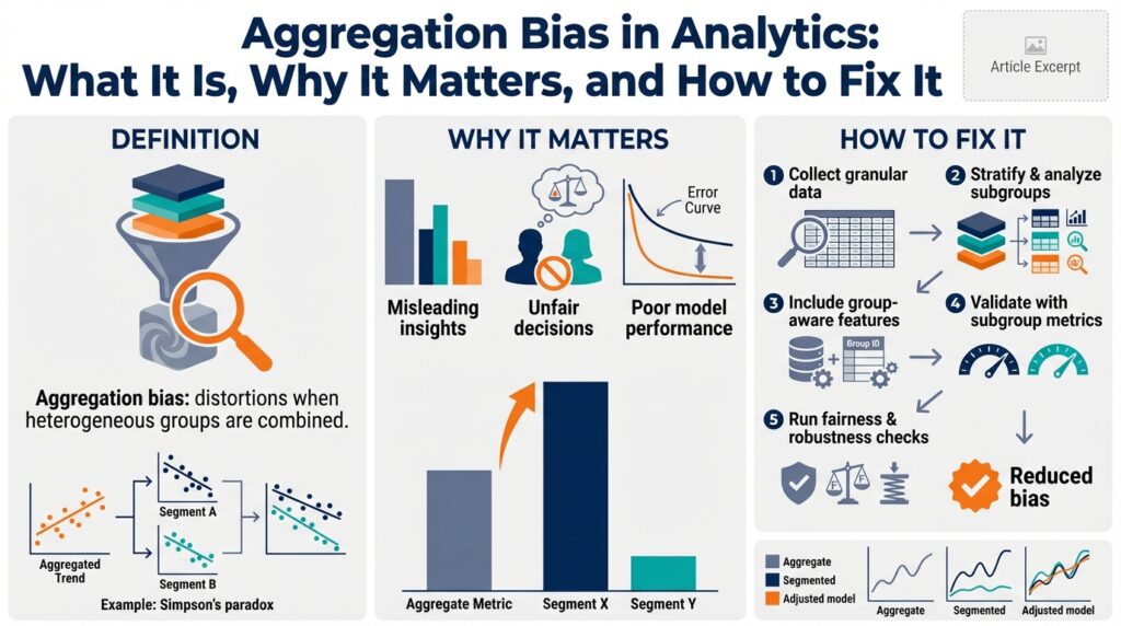
Building on this foundation, we need to be precise about what aggregation bias is and why it undermines analytics and data aggregation pipelines from the start. Aggregation bias occurs when combining observations across heterogeneous subgroups produces a misleading summary statistic that does not represent any underlying subgroup accurately. In analytics work this shows up when a single dashboard metric or training label masks systematic differences between cohorts—leading you to optimize for the wrong objective or draw incorrect causal conclusions.
At its core, aggregation bias is a mismatch between the level of measurement and the level of inference. Aggregation (the process of summarizing many records into a single number) sacrifices information about variance and structure; bias (a systematic deviation) introduces consistent error when the omitted structure matters. For example, if user behavior differs by device type or geography, computing a single conversion rate without accounting for those factors creates an aggregated metric that systematically misrepresents most groups. This is the same statistical phenomenon behind Simpson’s paradox, where grouped trends reverse when data are combined.
We can make this concrete with a short numbers example so you see the mechanics. Suppose Region A: 20 conversions out of 200 visitors (10%), Region B: 80 conversions out of 400 visitors (20%). Aggregated across both regions we get 100/600 = 16.7%, which understates Region B and overstates Region A; if your product changes only affect Region B you’ll mis-evaluate the impact when looking at the global metric. That mismatch between per-group signals and the global statistic is what creates bad decisions in dashboards, A/B tests, and KPIs.
This matters across engineering workflows, not just reporting. In model training, label aggregation or poor sampling can produce models that perform well on the global test set but fail for important cohorts; in monitoring, global alert thresholds hide failing subpopulations; in prioritization, product teams prioritize features that improve the averaged metric while harming specific user segments. Consequently, aggregation bias can introduce technical debt: fixes that appear to work broadly but degrade experience for critical slices of your user base.
How do you spot aggregation bias before it costs you? Start by asking: when should we trust a global metric, and when should we inspect subgroups? Run stratified analysis early—split by obvious axes like region, device, entry channel, or customer tier. Visualize distributions (box plots, decile plots) rather than just means, and compute per-group effect sizes and confidence intervals. If group-level estimates vary substantially or show different trends over time, the global metric is suspect and further decomposition is warranted.
When you confirm aggregation bias, choose mitigation strategies that match the problem scale and team constraints. For operational dashboards, publish both global and per-cohort metrics and weight alerts by criticality. For statistical inference, use multilevel (hierarchical) models or mixed-effects models to pool information across groups while preserving group-level estimates. For machine learning, adopt stratified sampling for training/validation, include group identifiers as features, and evaluate metrics by cohort rather than only globally.
Consider a real-world engineering scenario: a recommendation system trained on an aggregated click-through rate. After a release, overall CTR rises slightly but retention drops among a premium customer segment. By running per-segment validation and training a hierarchical model that captures segment-specific intercepts, we can detect and correct for the premium segment’s divergent behavior without retraining entirely separate models. We also instrument per-cohort monitoring so regressions are caught early and rollout can be gated by slice-level performance.
Recognizing aggregation bias changes how we design metrics, build models, and run experiments: we stop treating the global number as the single source of truth and instead adopt a layered view of insights. As we move to mitigation techniques and implementation patterns next, keep in mind that disaggregation and appropriately modeled pooling are the central levers for turning biased aggregates into actionable, trustworthy analytics.
Causes and Paradoxes
Building on this foundation, aggregation bias often arises from design choices that flatten meaningful heterogeneity into a single number. When you summarize across diverse cohorts—different geographies, device families, acquisition channels, or customer tiers—you remove the structure that explains why behavior differs; that removal is the primary cause of aggregation bias. In production analytics, the root causes are usually practical trade-offs: limited instrumentation, storage or query cost concerns, and dashboards designed for simplicity over nuance. These operational constraints push teams toward coarse aggregates that mask systematic differences and create persistent blind spots in decision-making.
A second common cause is model and label construction that ignores subgroup-specific processes. If you create a training label or KPI by collapsing multiple outcomes into one target without conditioning on known axes of variation, your model learns an average objective that may not align with any subgroup’s true objective. For example, labeling churn only as a binary global outcome can hide different churn drivers across cohorts; models then allocate capacity to patterns that reduce overall loss but fail where it matters. This mismatch between the level of modeling and the level of behavioral heterogeneity is a canonical source of technical debt in ML systems.
What causes aggregation bias in practice? Often it’s statistical convenience and human heuristics—people prefer single numbers and clear narratives—combined with non-random sampling. Non-random sampling means some cohorts are over- or under-represented in the aggregate, skewing the summary. This is precisely the mechanism behind Simpson’s paradox, where a trend that holds inside each subgroup reverses when combined. Simpson’s paradox is not merely a curiosity; it signals that confounding or differing baseline rates exist across groups and that the aggregate estimate is not causally interpretable without additional conditioning.
To develop intuition, think in terms of weighted mixtures and omitted-variable bias. An aggregate metric is a weighted average of subgroup statistics where weights are the subgroup sizes or exposure. If subgroup behaviors and subgroup prevalences both change—say, a growth channel brings many low-converting users—the aggregate can move even though each subgroup’s conversion probability is stable. Conversely, if an intervention affects only a small but high-value cohort, its impact may be invisible in the global average. This mathematical interplay of weights and subgroup-specific parameters explains why aggregation bias produces paradoxical outcomes and why raw averages can be misleading for operational decisions.
In engineering workflows, these causes create specific paradoxes you’ll recognize: A/B tests that pass globally but fail in a critical segment, monitoring alerts that stay silent while a minority cohort degrades, and feature prioritization that optimizes average engagement at the expense of retention for power users. For instance, when you stratify by signup source or API client version, you often discover opposite treatment effects; the global “winner” can be a loser for high-ARPU or enterprise users. These paradoxes matter because product changes are rolled out based on the global metric, leading to regressions for the groups whose behavior actually defines long-term value.
Taking this concept further, you’ll need to balance disaggregation with statistical power: disaggregate too finely and estimates become noisy; aggregate too much and you hide bias. Therefore, we typically combine cohort analysis with principled pooling—hierarchical models or regularized per-group estimates—and guardrails like minimum sample thresholds and cohort-level significance checks. As we move to mitigation patterns, remember the cause-and-effect relationship: address the data collection and labeling causes first, then apply modeling techniques that respect subgroup structure so you avoid repeating the same paradoxes in downstream systems.
Examples and Risks
Building on this foundation, we’ll make aggregation bias concrete with examples you’ll see in day-to-day analytics and engineering work. Start by treating the global metric with healthy skepticism: a single conversion rate, retention number, or model accuracy often hides heterogeneous behavior across cohorts. Aggregation bias and analytics are front-loaded here because if you rely on a single summary to steer product, ops, or ML decisions, you’re optimizing a blended objective that may not match any real user group. This section shows concrete failure modes and the operational risks that follow.
A common product example is acquisition-channel mixing that masks campaign performance differences. Suppose organic users convert at 8% while paid-search converts at 18%, but a surge in low-value paid traffic doubles the paid cohort size; your overall conversion moves closer to 14% and you might conclude growth is healthy. That global view hides the fact that retention for organic users—who may be higher lifetime-value—is falling. In practice you should run cohort-level evaluation (by campaign, entry page, or referral source) and treat aggregate conversion as a high-level signal, not the definitive KPI for prioritization or rollouts.
In machine learning, aggregation bias appears when labels or objectives collapse distinct generative processes into a single target, producing models that underperform for important slices. A fraud detection model trained on mixed geographies can learn spurious signals that work on the majority country but fail on smaller markets, causing elevated false positives there. To detect this, evaluate performance by cohort and compute per-group precision/recall. Techniques like stratified sampling, group-aware cross-validation, and adding group identifiers as features reduce this risk while preserving global utility.
Operational monitoring suffers similar blind spots: global alert thresholds and averaged latency percentiles can remain green while a particular API client version or region degrades. For example, a new SDK rollout that affects only 7% of traffic can trigger repeated errors for a high-value customer segment without moving the system-wide p95. This creates missed SLAs and slower incident detection. Instrument per-client-version and per-region metrics, and surface slice-level alerts when a slice crosses business-critical thresholds to avoid silent failures.
Causal and experimental risks are acute: A/B tests can pass on the global metric while harming segments you care about—a classic manifestation of Simpson’s paradox in product experiments. How do you know when an A/B test winner is misleading? Pre-specify slices for analysis, test for treatment-by-group interactions, and require slice-level sanity checks before full rollout. If treatment effects differ across pre-identified cohorts, treat the experiment as heterogenous rather than universally successful; that distinction should change rollout strategy and risk tolerance.
There are trade-offs between statistical power and fidelity: disaggregate too far and estimates become noisy; aggregate too much and you reintroduce bias. Practical mitigations include hierarchical (multilevel) models and regularized per-group estimates that pool information while preserving group-level variation, minimum-sample thresholds for reporting, and gated rollouts that validate slice-level metrics. For quick checks, run cohort SQL like SELECT cohort, COUNT(*) AS n, AVG(conversion) AS conv FROM events GROUP BY cohort to reveal the weight-and-rate interplay that creates biased aggregates.
Recognizing these examples and risks changes how we instrument, model, and run experiments: we stop treating aggregated metrics as final answers and instead adopt layered reporting, slice-aware validation, and model structures that respect subgroup heterogeneity. Next, we’ll map these diagnostic patterns to concrete implementation techniques—how to collect the right telemetry, choose pooling priors, and automate slice-level alerts—so your analytics and models reflect the realities of diverse user behavior rather than an averaged illusion.
How to Detect Bias
Aggregation bias can hide itself inside a clean-looking global KPI, so detecting it early is critical for trustworthy analytics and model validation. Start by assuming the global number is informative but incomplete: run cohort analysis and per-group diagnostics as part of every dashboard, experiment, and model validation step. How do you spot aggregation bias before it costs you? We’ll walk through repeatable checks—statistical, visual, and operational—that surface heterogeneity and show when a single aggregate is misleading.
Building on this foundation, the first practical check is systematic stratification: split your metric across obvious axes such as region, device, acquisition channel, API client version, or customer tier. Compute per-cohort rates and sample sizes and compare effect sizes rather than raw percentages, because relative differences matter more than absolute movement in noisy slices. For a quick SQL sanity check use a grouped summary that includes counts and dispersion, for example: SELECT cohort, COUNT(*) AS n, SUM(conversion)::float/COUNT(*) AS conv_rate, STDDEV_POP(conversion) AS sd FROM events GROUP BY cohort; — large differences in conv_rate with non-overlapping confidence ranges are a red flag.
Next, treat heterogeneity like a statistical hypothesis to test rather than an aesthetic observation; run interaction tests and variance-partitioning to quantify how much outcome variance is explained by group membership. Fit a simple regression with group and treatment interaction terms and test whether the interaction coefficients are significant — if they are, the treatment effect depends on cohort. We can also inspect heterogeneity metrics (for example, percent variance explained by groups) to prioritize which slices to investigate further and to decide whether pooling or disaggregation is required.
Visual diagnostics reveal patterns numbers hide. Plot small multiples of time-series metrics by cohort, overlay per-group confidence bands, or use decile plots and cumulative distribution functions to compare distributions rather than only means. Specifically, a small-multiples grid of conversion-rate time series will show divergent trends that a single global line smooths over, and density plots expose multi-modality that suggests distinct subpopulations. Visual checks are fast, communicate risk to stakeholders, and often reveal which cohorts drive aggregate movement.
Automate slice-level monitoring so detection scales with product changes: instrument slice-specific metrics, enforce minimum-sample thresholds to avoid chasing noise, and raise alerts when a slice’s metric crosses a business-critical boundary or diverges from a hierarchical baseline. Implement rolling-window comparisons (week-over-week or pre/post-rollout) per cohort and trigger an investigation when the slice effect exceeds a pre-specified delta. This operational approach prevents silent failures where the global p95 or average stays within bounds while a high-value cohort degrades.
For machine-learning pipelines, incorporate cohort-aware validation: produce per-group confusion matrices, precision/recall curves, and calibration plots in your model validation report. Use stratified holdouts or group K-fold cross-validation so that each fold preserves cohort structure, and compute metrics like AUC or F1 per cohort to detect models that perform well on average but poorly for specific users. If you use automated model monitoring, baseline per-cohort performance and alert on drift or sudden drops in cohort-level metrics rather than only global metrics.
Finally, adopt pragmatic decision rules to balance noise and fidelity: disaggregate when cohorts are business-critical or when interaction tests indicate heterogeneous effects, otherwise use hierarchical models or regularized per-group estimates to pool information while preserving subgroup signals. Gated rollouts that require slice-level sanity checks before full launch reduce risk when you find meaningful heterogeneity. These rules help you decide when to act on a cohort signal, when to model it explicitly, and when to accept aggregated reporting with clear caveats.
Detecting aggregation bias is a reproducible engineering discipline: combine stratified summaries, interaction tests, visual inspections, automated slice-level monitoring, and cohort-aware validation so we can surface heterogeneity reliably. With those checks embedded in dashboards, experiments, and model pipelines, you’ll catch the misleading aggregates early and choose mitigation strategies that preserve both statistical power and real-world fidelity.
Fixes: Disaggregate and Stratify
Building on this foundation, start by treating aggregation bias as a signal that you must disaggregate your metrics and stratify analysis along the axes that matter most to the business. We want the term aggregation bias in the first lines because it sets the problem context: a global metric can hide divergent cohort behavior and drive the wrong decisions. If you suspect heterogeneous treatment effects or shifting sample weights, prioritize slicing by obvious dimensions—region, device family, signup source, API client version, or customer tier—so you can see whether the global number reflects any real subgroup.
When should you disaggregate versus pool information? Use disaggregation when the subgroup is business-critical, when treatment-by-group interactions are statistically significant, or when a subgroup’s behavior drives long-term value (for example, premium users or enterprise accounts). Splitting makes sense early in experiments and post-release monitoring because it surfaces regressions that global averages obscure. However, we also acknowledge the trade-off: smaller slices increase variance, so disaggregation must be paired with rules for minimum sample sizes and practical significance tests.
Operationally, install stratification into your data pipeline so cohort-aware summaries are produced automatically alongside global KPIs. For example, emit daily grouped summaries like SELECT cohort, COUNT(*) AS n, AVG(conversion) AS conv_rate FROM events GROUP BY cohort; and compute confidence intervals or Bayesian credible intervals per group. Enforce a minimum n threshold before surfacing a slice to downstream dashboards, and tag slices as “watch” or “stable” based on variance and business impact. This makes cohort analysis a first-class output of ETL, not an ad-hoc investigation.
For modeling, prefer hierarchical (multilevel) models when you need both per-group estimates and statistical power. A random-intercepts model pools information across groups while shrinking noisy slice estimates toward the global mean, which reduces false alarms without erasing real heterogeneity. When you need interpretability, fit a mixed-effects regression with group-specific intercepts and treatment interactions; when production constraints demand speed, implement empirical Bayes shrinkage or regularized per-group logistic regressions as pragmatic approximations.
In machine-learning pipelines, maintain cohort fidelity in training and validation. Use stratified sampling or GroupKFold cross-validation so that folds respect group boundaries (for scikit-learn: GroupKFold(n_splits=5).split(X, y, groups)). Include stable group identifiers as features if they capture causal heterogeneity, but beware of leaky identifiers that proxy for label information. Always report per-cohort metrics—precision, recall, calibration plots—so you can detect models that perform well on average but fail for important slices.
Monitoring and rollout practices must reflect the disaggregated reality you now measure. Gate rollouts with slice-level acceptance criteria and run canary releases that target representative cohorts before full rollout. Configure alerts to trigger when a slice crosses a business-critical threshold rather than only when the global metric shifts; for instance, fire an incident if premium-user retention drops by X% or if any client-version error rate exceeds Y. These operational controls turn cohort signals into actionable checkpoints.
How do you pick the right granularity for stratification? Start with hypothesized causal axes and business priorities, then iterate based on signal-to-noise: merge low-impact tiny slices, and split large, heterogeneous cohorts. Apply automated rules—minimum sample size, persistent effect across windows, and alignment with product ownership—to decide which slices stay in permanent reporting. This governance balances statistical power with fidelity so you don’t chase random fluctuations.
Taking these steps changes how we instrument, model, and operate analytics: we stop trusting a single aggregate and instead create layered, cohort-aware insight that reduces aggregation bias while preserving power. In practice that means automated stratified summaries, hierarchical modeling where appropriate, cohort-aware ML validation, and gated rollouts that protect high-value users. Next we’ll look at how to choose pooling priors and automate slice-level alerts so your pipelines keep detecting heterogeneity as traffic and product mix evolve.
Implementing Fixes in Pipelines
Building on this foundation, the first thing to accept is that aggregation bias must be treated as an engineering problem inside your data and model pipelines, not an occasional analytics footnote. If you want reliable cohort analysis and trustworthy KPIs, you have to bake slice-aware computation, validation, and gating into ETL, model training, and monitoring. Treating aggregation bias as a cross-cutting concern forces you to instrument at the right granularity and to make cohort-level outputs first-class pipeline artifacts rather than ad-hoc reports.
Start at the ingestion and ETL layer by emitting grouped aggregates and metadata alongside raw events. Design your data contracts so each event includes stable cohort identifiers (for example, region, client_version, acquisition_channel, customer_tier) and a provenance field for sampling decisions; this makes cohort analysis reproducible and debuggable. Compute daily or hourly grouped summaries as native outputs of your pipeline and persist count, mean, variance, and a stability flag (minimum-sample or effective-sample) so downstream jobs can decide whether to act on a slice.
How do you enforce minimum-sample rules and surface noisy slices automatically? Implement deterministic thresholds in your pipeline and surface confidence intervals in reports. For example, a simple grouped SQL job can run as part of ETL:
SELECT cohort, COUNT(*) AS n, AVG(conversion)::float AS conv_rate,
  -- approximate 95% CI using normal approximation
  1.96 * SQRT(conv_rate*(1-conv_rate)/GREATEST(n,1)) AS ci95
FROM events
GROUP BY cohort;
Mark slices with n below the minimum as “insufficient” so dashboards and downstream model trainers treat them differently, and persist these flags so monitoring can trend sample sufficiency over time.
In training pipelines, preserve cohort fidelity with stratified sampling and group-aware CV so your model validation reflects real heterogeneity. Use GroupKFold or stratified samplers that guarantee each fold contains representative slices (for scikit-learn: GroupKFold(n_splits=5).split(X, y, groups)). Include group identifiers as features only when they are stable, non-leaky proxies for behavior; otherwise, prefer model structures that encode per-group variation explicitly.
When you need both per-group estimates and statistical power, integrate hierarchical models into your training or post-processing steps. Hierarchical models (multilevel models) let us pool information across slices while retaining group-specific intercepts or slopes; in practice we often implement them as a Bayesian model in training or as an empirical-Bayes shrinkage step applied to per-group estimates. If latency or engineering constraints prevent full Bayesian deployment, approximate pooling with regularized per-group regressions or an online shrinkage layer so you get most of the robustness of hierarchical models without a heavy runtime cost.
Operationalize slice-level monitoring and gated rollouts so fixes don’t just live in notebooks. Instrument slice-level metrics and expose them to your alerting system with business-prioritized thresholds—for example, require canary traffic to meet slice-level performance before unblocking a full rollout. Use feature flags and progressive rollouts that can be targeted by cohort, and configure automatic rollback rules when any critical slice crosses a pre-defined delta relative to its baseline. Cohort analysis should be part of your SLO definition for key user groups, not an afterthought.
Finally, treat tests and CI as your safety net: add unit tests that validate aggregated outputs, data-quality checks for cohort identifiers and sample counts, and synthetic regression tests that inject cohort-level shifts to ensure your alerts and model retraining triggers fire. Automate schema checks and drift detectors that compare current slice distributions to historical baselines and gate deployments when drift or sudden composition changes appear. Together, these pipeline-level practices stop aggregation bias from reappearing as silent technical debt.
Taking this concept further, automate governance so cohort-aware summaries, minimum-sample rules, hierarchical pooling choices, and slice-level alerts are configurable policy artifacts rather than buried scripts. When these controls are integrated into CI/CD, monitoring, and model training, you turn cohort analysis from an ad-hoc investigation into repeatable pipeline behavior that prevents aggregation bias from derailing decisions as traffic and product mix evolve.