Essential AI Terms and Concepts
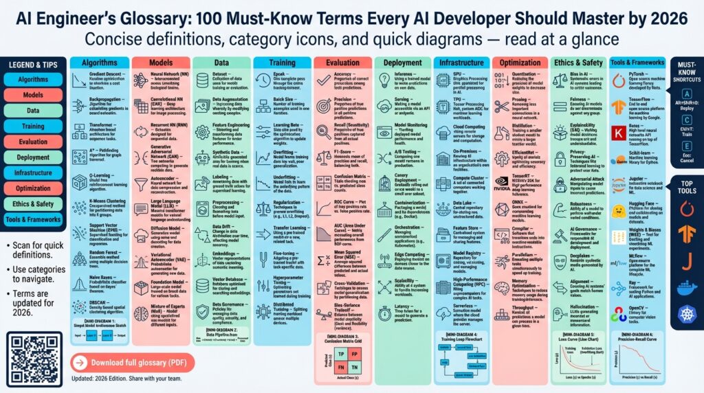
Building on this foundation, we need a compact shared vocabulary so you and your team can reason about trade-offs quickly. Start by treating a model as a mathematical function that maps inputs to outputs; in practice that function is parameterized by weights learned from data. For an AI engineer this framing clarifies why dataset quality and objective selection matter as much as architecture choices. Early concepts you should front-load in design conversations include dataset, loss function, generalization, and the distinction between machine learning and deep learning.
A dataset is more than rows and columns — it’s the signal your model will learn from and the bias it will inherit. Supervised learning assigns labels and minimizes a loss function (for example cross-entropy for classification), while unsupervised learning extracts structure without labels. The training loop uses gradient descent to update parameters by backpropagating loss; understanding the optimizer, learning rate schedule, and batch size is essential when tuning for convergence. For instance, an image classifier’s poor accuracy often traces back to label noise or class imbalance rather than the network topology.
Model capacity and generalization determine whether you underfit or overfit a problem, so we must measure and mitigate both. Regularization techniques—weight decay, dropout, data augmentation—lower variance; cross-validation and early stopping help validate that improvements generalize. Consider a small dataset scenario: transfer learning or parameter-efficient fine-tuning prevents overfitting by reusing pre-trained features. Monitoring train/validation gap and plotting learning curves are simple, high-utility diagnostics you should run before changing model size.
Architectural choices matter: convolutional networks still dominate vision, transformers power sequence tasks, and embeddings turn discrete inputs into dense vectors for retrieval or semantic search. Transfer learning and fine-tuning adapt foundation models to domain tasks; parameter-efficient methods like LoRA or adapters let you tune large language models (LLMs) without full-weight updates. A typical pattern is: initialize with pretrained weights, freeze early layers, and train a small adapter block — this reduces training cost and preserves pretraining knowledge. Embeddings also let you decouple semantic search from generation by using nearest-neighbor indices.
When you move from prototype to production, performance constraints shift: inference latency, throughput, and cost become dominant factors for model deployment. How do you choose between batching for throughput and single-request latency? Use quantization to reduce model size and accelerate CPU inference, pruning to remove redundant parameters, and model distillation to create a lightweight student model for edge use. Also evaluate hardware trade-offs: GPUs or accelerators for batched high-throughput services, and optimized CPU paths for low-cost, low-latency endpoints.
Operationalizing models requires MLOps practices that mirror software engineering: reproducible pipelines, CI/CD for training and deployment, model registries for versioning, and automated monitoring for drift. Instrument both data and prediction distributions so you can detect concept drift and trigger retraining or rollback via canary deployments. In addition, integrate metrics for business impact (conversion lift, error cost) not just technical metrics; A/B tests and shadow traffic let you validate model changes safely before full rollout.
Evaluation must cover accuracy, calibration, fairness, and robustness simultaneously—no single metric tells the whole story. Use precision/recall/F1 where class imbalance matters, calibration curves to assess confidence, and adversarial tests or perturbation suites to probe brittleness. Include explainability diagnostics (for example SHAP) and privacy-preserving techniques like differential privacy when handling sensitive data. Taking this vocabulary and these checks into your next architecture discussion will let us move from conceptual models to deployable, auditable systems that meet real-world constraints.
Model Architectures: Transformers and Beyond
Building on this foundation, the dominant paradigm for sequence and language tasks is the transformer, and understanding its design lets you reason about a wide spectrum of model architectures and their trade-offs. The transformer centers an attention mechanism that computes pairwise interactions between tokens, replacing recurrence with parallelizable matrix operations; this design is why transformers scale so well on modern accelerators. When we say “attention,” we mean the soft, learnable weighting of token pairs (queries, keys, values) that lets the model route context dynamically rather than via fixed receptive fields. Keep these core ideas in mind as you compare encoder-only, decoder-only, and encoder–decoder topologies for tasks like classification, generation, and translation.
At the implementation level, the attention pattern determines both capability and cost. Self-attention gives global context—useful for long-range dependencies—yet its O(n^2) memory with sequence length forces design choices for production: chunking, sparse attention, memory compression, or linearized attention approximations. Positional encodings restore order information that attention discards; causal (unidirectional) attention enforces autoregressive generation while bidirectional/masked attention supports contextual encoding. These distinctions matter when you select a pretraining objective: masked language modeling yields strong encoders, autoregressive objectives produce fluent decoders, and the hybrid choices influence how you fine-tune or deploy a foundation model.
Scaling transformers changes the game, but it also shifts bottlenecks from algorithmic to systems problems. Bigger models improve few-shot learning and transfer but amplify inference latency, memory, and cost—so we routinely trade dense capacity for conditional compute patterns like Mixture-of-Experts (MoE) to serve capacity selectively. MoE routes each token to a sparse subset of experts, lowering FLOPs per example while retaining a larger effective parameter count; however, MoE adds routing complexity, load balancing concerns, and sometimes degraded latency tail behavior. For long-context workloads or retrieval-heavy pipelines, supplementing the model with an external vector store or a key-value cache for past tokens reduces both computation and tokenization overhead during inference.
Beyond vanilla transformers, specialized model architectures address domain-specific inductive biases. For vision and multimodal work, convolutional backbones, equivariant networks (for 3D/physics-aware tasks), and diffusion models offer different trade-offs: diffusion excels at high-fidelity generative imaging, while vision transformers (ViT) simplify patch-based attention at the cost of needing larger datasets or stronger pretraining. Graph neural networks (GNNs) remain the right choice when relational structure dominates, and hybrid designs—such as graph transformers or conv-attention blocks—let you combine locality with global context. Retrieval-augmented generation (RAG) architectures pair a dense encoder and a retrieval index so the model conditions on external knowledge, improving factuality without enlarging weights.
In practice, you’ll mix architectural choices with parameter-efficient tuning and deployment strategies. Adapter layers, LoRA-style low-rank updates, and small gated modules let you adapt a large transformer to new domains without full-weight retraining—this reduces cost and preserves pretrained knowledge. On the systems side, model parallelism (tensor and pipeline), sharding, and 8-bit or quantized kernels are essential for serving large architectures with acceptable latency and throughput. Design your training and inference pipelines so you can swap between dense and sparse compute paths depending on SLA: batch-heavy offline scoring favors different sharding than single-request, low-latency interactive services.
When should you pick an MoE or a dense transformer, or combine retrieval with a compact decoder? The short answer is: choose based on workload patterns—if you need peak capacity for a wide range of rare queries, MoE or retrieval-augmented models make sense; if you need predictable latency and simpler infra, a distilled dense transformer or a student model works better. Evaluate using task-specific probes (long-range dependency tests, multimodal alignment checks) and production metrics (p99 latency, cost per inference, calibration) to validate that the architecture meets both model quality and operational constraints.
Taking these patterns together, architects should treat transformers as a flexible substrate rather than a monolith: attention gives you a programmable communication layer, and the right architectural extensions—sparsity, retrieval, equivariance, or diffusion—let you tailor capability to domain requirements. As we move from prototyping to production, explicitly map the model’s computational graph to your deployment stack and choose the sparsity, parallelism, and tuning patterns that align with your SLAs and data constraints. Next, we’ll examine how to evaluate robustness and calibration across these architectures so you can compare models on more than just raw accuracy.
Data Management and Preprocessing Best Practices
Building on this foundation, strong data management and clear data preprocessing choices are the single biggest levers for reliable model behavior and faster iteration. If your dataset is noisy, unversioned, or riddled with silent schema changes, model changes will feel like guesswork rather than engineering. How do you turn messy inputs into a reproducible, auditable training signal that preserves privacy and supports quick experimentation? We’ll walk through practical patterns—proven data pipeline practices, preprocessing best practices, and operational controls—that you can apply today.
Start by treating provenance and dataset versioning as first-class engineering artifacts. Provenance means recording where each sample came from, when it was ingested, and which transform produced it; dataset versioning captures immutable snapshots tied to a model training run. These concepts let you reproduce training exactly, roll back to a prior snapshot when a regression appears, and trace label quality issues back to their source. For example, store a content hash for each file and keep a metadata table with ingestion timestamps and schema version—this makes debugging label drift and upstream API changes tractable.
Focus cleaning and label hygiene on measurable rules rather than ad hoc fixes. Implement deterministic deduplication (e.g., df.drop_duplicates(subset=[“id”]) or hashing-based nearest-neighbor for fuzzy dedupe), validate label distributions with automated tests, and flag outliers with statistical rules or lightweight isolation-forest detectors. Define label guidelines and a review workflow for edge cases: when multiple annotators disagree above a threshold, push those samples into adjudication instead of retrying blind relabeling. When you encounter class imbalance, prefer targeted augmentation or stratified resampling over wholesale oversampling, and always hold out a stratified validation set so your metrics reflect class-wise performance.
Design your preprocessing pipeline for composability and idempotence. Encapsulate tokenization, normalization, encoding, and feature transforms as versioned, deterministic functions so the exact preprocess used during training can be re-run at inference. Beware target leakage: never compute features that incorporate information from the future or the label—timestamp joins and rolling-aggregate leaks are common traps. For numerical pipelines, standardize using training-set statistics (mean, std) persisted to the feature metadata; for categorical variables use stable mapping tables or learned embeddings that degrade gracefully when unseen categories appear.
Automate quality gates in the data pipeline and integrate them with CI for model training. Implement schema checks, null-rate thresholds, cardinality monitors, and distribution checks that run on every ingest; reject or quarantine batches that violate contracts. Treat these checks as code: unit-test transformations, add integration tests that load a representative slice of production traffic, and record metrics like missingness rate or PSI (population stability index). Robust dataset versioning combined with automated checks prevents surprises when a downstream feature changes format or an upstream vendor alters an API.
Operationalize privacy, access controls, and monitoring alongside preprocessing. Apply differential-privacy-aware aggregation for sensitive signals, enforce role-based access to raw data, and log data access for audits. Monitor data drift and concept drift with concrete metrics—KL divergence or earth mover’s distance for continuous features, label-distribution shifts for supervised tasks, and simple histograms for cardinality changes—and set p99 alert thresholds that trigger data investigation or retraining. For fairness, instrument subpopulation slices early and include sampling strategies to ensure underrepresented groups are included in training and validation.
When you design model training loops, treat the dataset and preprocessing pipeline as part of the model contract. Persist transform artifacts (scalers, vocabularies, embedding tables) alongside a dataset snapshot and the training config so we can reproduce a run months later. These practices reduce experimentation cost, make ablation studies credible, and let you move from flaky research prototypes to production systems with predictable behavior. In the next section, we’ll apply these data guarantees to evaluate robustness and calibration across architectures so you can compare models on more than just headline accuracy.
Training Strategies, Optimization, Regularization Techniques
Building on this foundation, the choices you make during model training determine whether a project ends with a deployable, robust system or a brittle experiment. Start by framing the problem: do you need rapid convergence on a new domain, predictable calibration for high-stakes decisions, or minimal inference cost at scale? That framing guides your training strategy selection and sets trade-offs for optimization and regularization. How do you pick the right approach when time, compute, and data quality all pull in different directions?
When data is limited or labels are noisy, favor transfer and parameter-efficient approaches first. Initialize from a pretrained checkpoint, freeze most of the backbone, and train a small head or adapter block with a conservative learning rate; this preserves pretrained features while reducing overfitting risk. For domain shifts, progressively unfreeze layers and apply discriminative learning rates—lower for early layers, higher for task-specific heads—so you retain generic representations while adapting task-specific features. We often use LoRA or adapter layers when full fine-tuning is too costly, since they let you iterate quickly and keep a small storage footprint for many downstream tasks.
Optimization choices control how fast and stably you reach a good solution, so treat the optimizer and schedule as core design decisions rather than tuning knobs. AdamW remains a reliable default for transformers and convnets because it decouples weight decay from adaptive moments; use SGD with momentum for vision tasks where large-batch training and sharp minima concerns matter. Combine a warmup phase (linear or cosine) with an annealing schedule—warmup for 500–5k steps depending on batch size, then cosine or linear decay—to avoid early instability and to improve final generalization. If you must train with small GPUs, use gradient accumulation to emulate larger batch sizes while monitoring effective batch-size effects on generalization.
Regularization techniques reduce variance and improve out-of-distribution behavior, but choose them deliberately based on dataset and objective. Weight decay penalizes large parameters and complements adaptive optimizers; dropout and stochastic depth add per-example noise that helps generalize, especially in overparameterized nets. Data augmentation (including mixup and RandAugment for vision or span masking for text) injects realistic variability into the signal and often beats heavy architectural changes when data is scarce. For classification, label smoothing can hedge overconfident outputs and improve calibration; combine it with explicit calibration checks to ensure it actually helps your metric of interest.
Put these pieces together into a reproducible recipe you can iterate on. Start with a short calibration run: freeze the backbone, train adapters or heads for a few epochs with lr≈1e-4 and weight_decay≈1e-2, evaluate validation curves, then unfreeze selectively and reduce the learning rate by an order of magnitude. Add early stopping with patience tuned to your noise level and log train/validation losses, precision/recall per-class, and a calibration metric. When switching from prototyping to production, run a distillation step or quantization-aware training to produce a student model with comparable accuracy but lower latency and memory footprint.
Diagnose problems with targeted signals rather than blind hyperparameter sweeps. If you see a growing train/validation gap, increase regularization, augmentations, or reduce effective model capacity; if both losses plateau high, either increase capacity or improve optimization with longer schedules or different optimizers. Monitor gradient norms, loss variance across mini-batches, and per-layer learning dynamics—exploding gradients often indicate rate issues while stagnant small gradients point to poor conditioning or saturation. Use budget-aware search (random search or Bayesian optimization) to tune the most impactful hyperparameters—learning rate, weight decay, and augmentation strength—rather than trying to tune every knob.
Taking these practices together, we trade opaque heuristics for a disciplined loop: choose an initial training strategy based on data and constraints, pick optimization methods and schedules that stabilize convergence, and apply regularization targeted to the observed failure modes. In the next section we’ll connect these training choices to robustness and calibration checks so you can validate that improvements hold across slices and deployment scenarios.
Evaluation Metrics, Validation and Robustness
Evaluation metrics, validation, and robustness are the levers that turn a promising prototype into a trustworthy system, and you should front-load them early in every project. When we say evaluation metrics, we mean the concrete numeric objectives you will optimize and monitor; when we say validation, we mean the experimental protocols that estimate generalization; and when we say robustness, we mean performance under realistic perturbations and adversarial conditions. Treat these three as a contract between model quality and production risk so you can make repeatable decisions about model changes, rollouts, and retraining windows.
Choosing the right evaluation metrics starts with the business objective and the data distribution. Precision, recall, and F1 score are appropriate when class imbalance matters and false positives versus false negatives have asymmetric costs; ROC AUC and PR AUC measure discrimination but answer different questions—use PR AUC for rare positive classes. Calibration metrics such as Brier score and Expected Calibration Error (ECE) matter when you make downstream decisions from predicted probabilities, and confusion matrices help you pick operational thresholds. How do you choose the right metric for a business objective? Map the metric to cost (monetary, safety, user trust), and select one primary metric plus a small set of secondary metrics to avoid metric hacking.
Validation is more than a train/validation/test split; it’s the experimental design that gives you confidence in reported metrics. For cross-sectional tasks use stratified K-fold to preserve label proportions, and for hyperparameter-heavy workflows adopt nested cross-validation to get unbiased performance estimates. For temporal or streaming data implement rolling-window or anchored backtesting to avoid target leakage and optimistic bias: hold out contiguous time ranges during evaluation and simulate the ordering you’ll see in production. Always persist the exact dataset snapshot and preprocessing artifacts used for each validation run so we can reproduce failures and perform targeted ablation.
Robustness testing should be deliberate, automated, and diverse in scope. Run adversarial perturbation suites (for example, projected gradient descent variants) to probe worst-case inputs, and run corruption or shift benchmarks—noise, blur, format changes, or upstream API alterations—to measure degradation under realistic failure modes. For NLP pipelines include paraphrase, synonym substitution, and tokenization-fuzzing tests; for vision include ImageNet-C–style corruptions or synthetic occlusions. Complement these with randomized stress tests and domain-split evaluations that surface brittle behavior across subpopulations.
Uncertainty quantification and calibration are practical levers for risk-sensitive systems. Use temperature scaling or isotonic regression to recalibrate model probabilities post-training, and consider ensemble methods or Monte Carlo dropout for predictive uncertainty estimates when you need epistemic uncertainty. For classification tasks, plot reliability diagrams and compute ECE to validate whether confidence percentiles align with empirical accuracy. If your downstream logic gates execution on a confidence threshold, prioritize calibration over raw accuracy so your operational decisions remain consistent.
Fairness and slice-based analysis belong to the same evaluation pipeline as technical metrics and robustness tests. Compute group-level metrics (demographic parity, equalized odds) alongside per-slice precision/recall and track intersectional slices to reveal hidden regressions. When you detect disparities, quantify the trade-offs explicitly: does improving one subgroup’s recall materially reduce overall precision or increase false alarms? Use constrained optimization or post-processing thresholds when necessary, and record the mitigation strategy and its impact in the model registry.
Make these checks part of CI/CD and the monitoring stack so validation becomes continuous rather than episodic. Automate a smoke-suite that runs core metrics, calibration checks, adversarial probes, and data-drift detectors (KL-divergence, PSI) on each candidate model; gate rollouts behind canary analyses or shadow traffic experiments that compare new and incumbent models on live inputs. Define clear alert thresholds and retraining triggers tied to business impact, not just statistical drift, so we act on degradation before it affects users.
A practical workflow ties these pieces together: pick a primary evaluation metric aligned with business cost, design a validation protocol that matches deployment ordering, run robustness suites and calibration procedures, then codify the successful recipe into CI gates and production monitors. For example, when deploying an image classifier for QA automation we might optimize PR AUC, validate with stratified temporal splits, run corruption and adversarial tests, apply temperature scaling, and only promote models that pass a shadow-traffic fidelity check. This integrated loop turns isolated experiments into auditable, repeatable releases.
Taking these practices together, treat metrics, validation, and robustness as a unified engineering discipline rather than separate checklists. By choosing metrics that reflect real costs, validating with protocols that mirror production, and stress-testing models against realistic perturbations, we reduce surprise in deployment and improve decision-making under uncertainty. In the next section we’ll connect these evaluation practices to architecture-specific checks so you can compare models on calibration, fairness, and resilience across design choices.
Deployment, Monitoring, and MLOps Workflows
Building on this foundation, the operational gap between a validated model and reliable production service is where many projects fail—so prioritize deployment, monitoring, and MLOps workflows from day one. You should treat deployment as a repeatable engineering pipeline, not an ad hoc script: that means versioned artifacts, a model registry that ties checkpoint, dataset snapshot, and preprocessing artifacts to a single immutable release, and CI/CD gates that run quality checks before any production change. When we design this pipeline, we focus on reproducibility, auditability, and the business metrics that matter; those priorities guide how you construct every step of the workflow and the metrics you expose to stakeholders. Early investment here reduces firefighting later when drift or regressions surface in live traffic.
Start by defining the core components of an MLOps workflow and the contracts between them: source control for code and configs, an automated training pipeline that produces signed artifacts, a model registry for versioning and metadata, and deployment runners that know how to map a model artifact to an environment. The model registry is more than storage—it’s the source of truth for lineage, approvals, and reproducibility; attach evaluation reports, calibration artifacts, and fairness checks to each entry so you can gate promotion. CI/CD for models must include not only unit and integration tests but also a smoke-suite of model-specific checks (sanity, calibration, basic adversarial probes) that run automatically on pull requests and candidate releases. Treat these pieces as code: automate them, test them, and make rollbacks predictable.
Choose deployment patterns that match your SLA and traffic profile rather than defaulting to one architecture. For interactive, low-latency services we often use GPU-backed endpoints with autoscaling and request batching to balance p99 latency and throughput; for asynchronous batch scoring, container orchestration or serverless batch jobs reduce cost and complexity. How do you decide between canary, blue–green, and shadow deployments? Use canaries and gradual rollouts when you need live validation against a small slice of real traffic; use shadow traffic or A/B experiments when you want fidelity checks without impacting users. Container orchestration tools and inference servers give you the operational primitives (health checks, readiness probes, resource limits) you need to make these patterns robust.
Monitoring and observability must measure both technical health and business impact so alerts signal meaningful degradation rather than noise. Instrument prediction latency, error-rate, resource metrics, and calibration statistics alongside data-distribution metrics for key features; collect separate channels for label feedback so you can compute live accuracy when ground truth arrives. Implement drift detection for input and prediction distributions (for example, PSI or KL-divergence) and set pragmatic thresholds that trigger investigation or automated retraining pipelines. Build dashboards that correlate model signals to business KPIs so you can answer questions like whether a drop in conversion is due to model drift or an upstream data regression.
Automated retraining and governance close the loop but need guardrails. Define retraining triggers explicitly—data-volume thresholds, sustained drift windows, or monitored KPI slippage—and codify retraining pipelines that run in staging with the same tests as CI/CD before any promotion. Include human-in-the-loop approvals for high-impact changes, and keep rollback simple by promoting the previous registry entry if sanity checks fail. Capture lineage and explainability artifacts (feature importances, SHAP summaries) with each training run to support audits and fairness reviews; these artifacts let you diagnose regressions and justify decisions during postmortems.
A practical end-to-end workflow ties these concepts together: a commit triggers CI that runs unit tests and a model smoke-suite; a successful branch run spins up a training job that writes artifacts to the registry with evaluation metadata; a controlled canary deploy serves a fraction of traffic while monitoring calibration, latency, and business KPIs; if checks pass, automated promotion completes the deployment and monitoring continues to guard against drift. By automating these steps and exposing clear contracts between teams, you reduce cognitive load, speed iterations, and keep the system auditable—so we can iterate on models confidently rather than reactively. This operational discipline sets the stage for scaling models safely across products and teams.


