Why Distill Large Models
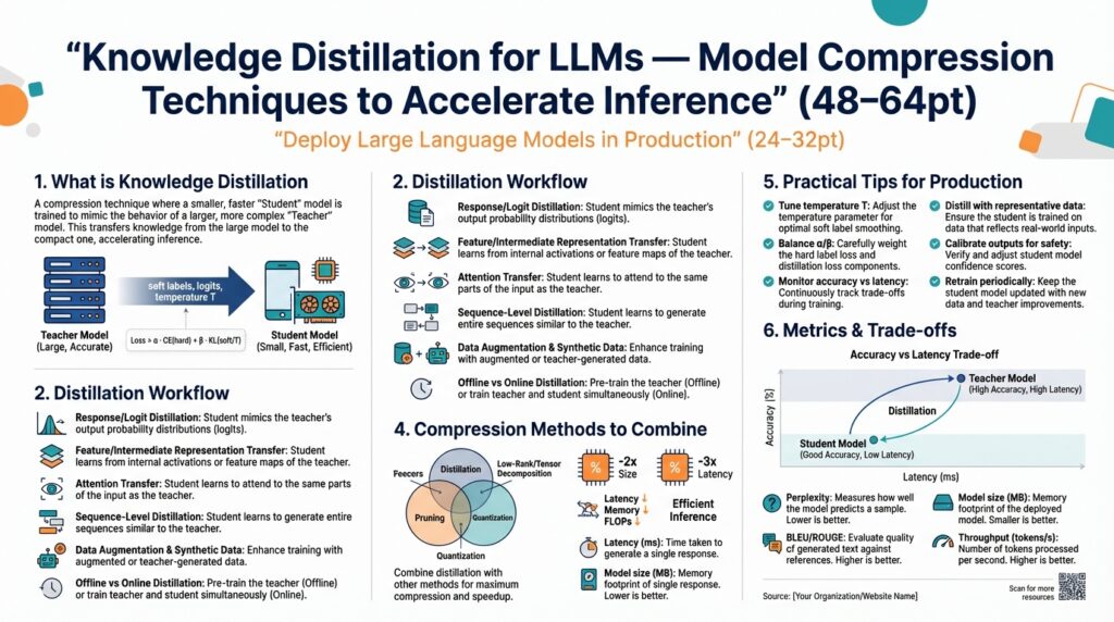
Knowledge distillation and model compression are the practical levers you pull when production constraints collide with the accuracy of large models. In the first 100 words we need to call out why you care: reduced inference latency, smaller RAM/VRAM footprints, and lower operational cost while keeping much of the teacher model’s capabilities. If you want to deploy large language models in production without provisioning clusters of expensive GPUs, knowledge distillation gives you a reproducible path from a high-performing teacher to a faster, cheaper student model.
Start with the trade-off: latency and cost versus capability. Large models deliver superior zero-shot reasoning and few-shot robustness, but their inference time and memory use make them impractical for many services—real-time APIs, on-device assistants, and edge deployments. Distillation compresses that capability into a smaller student by transferring behavior rather than re-training from scratch, so you preserve task performance for common workloads while cutting inference latency and throughput costs. This is why engineering teams prioritize distillation before spending on additional hardware or sharding complexity.
Mechanically, distillation is about what we match and how we train. The canonical approach is teacher-student learning where the student minimizes a combination of task loss and a distillation loss that matches teacher logits or softened probabilities; for example, loss = CE(student, labels) + α * KL(softmax(student_logits/T), softmax(teacher_logits/T)). Temperature T, the weighting α, and whether you match token-level logits, hidden states, or attention maps are levers you tune. For sequence models you can also use sequence-level distillation or response-level imitation (student generated outputs compared to teacher outputs) to preserve generation quality under autoregressive decoding.
You’ll face concrete engineering decisions when applying distillation in production. For instance, if you need a 10x throughput improvement you might distill a 70B teacher into a 7B student and then apply 4-bit quantization; the combined pipeline—distill then quantize—often outperforms naive quantization of the teacher because the student learns to be robust to lower-precision activations. In another scenario, task-specific distillation (fine-tuning the student on teacher-labeled task data) can give you near-teacher accuracy for domain-specific intents while keeping the student model small enough to host in a single inference container.
How do you decide which model compression strategy fits your production constraints? Ask three questions: What latency and memory envelope must your service meet? Which failure modes from the teacher are acceptable to lose? And how much labeled or unlabeled data can you cheaply generate using the teacher? If low-latency is critical and you can generate teacher outputs at scale, aggressive distillation with response-level matching plus post-distillation pruning yields the best balance of accuracy and resource use. If you must preserve complex reasoning, consider hybrid architectures—route hard queries to the teacher and use the distilled student for the rest—to trade a small routing overhead for overall cost savings.
Distillation also improves operational robustness and observability. A smaller student is easier to deploy across regions, instrument for latency percentiles, and integrate into autoscaling policies, which reduces blast radius when you iterate on model updates. Moreover, students are easier to secure for on-device use because their footprint reduces attack surface vectors tied to memory and state. As we move to productionize large language models, treating knowledge distillation as a core model compression and deployment strategy gives you deterministic performance, lower cost, and a clearer upgrade path from research prototypes to stable services.
Distillation Types and Variants
Building on this foundation, the important practical question becomes which distillation variant to use for a given production constraint. Knowledge distillation and model distillation are umbrella terms, but they hide meaningful differences in what you match (logits, representations, behaviors) and how you train (token-level, sequence-level, or response-level). Picking the right variant directly affects latency, robustness to quantization, and how well the student preserves the teacher’s reasoning—so we need to be deliberate rather than defaulting to vanilla logits matching.
Logit-level distillation is the canonical, low-friction option: you soften teacher logits with a temperature and minimize a KL or MSE loss against student logits during token prediction. This approach works well when your priority is preserving per-token probabilities and when you have abundant teacher-generated text. For autoregressive LLMs it’s straightforward to implement inside your training loop and tends to produce compact students that retain surface-level fluency and calibration; however, it can miss deeper internal behaviors like multi-step reasoning.
Representation or hidden-state distillation moves beyond outputs to match intermediate activations, attention maps, or layer-wise features. We use this when the teacher’s internal computation pattern matters—for example, when the ability to chain multi-hop inference or maintain long-range context is critical. In practice you add auxiliary losses that align specific layers: loss = CE(student, labels) + α * KL(tokens) + β * L2(student_hidden_i, teacher_hidden_j). This variant requires careful layer mapping (projection layers often help when student and teacher sizes differ) and can yield students that generalize better on reasoning benchmarks.
Sequence-level and response-level distillation operate at a higher abstraction: you train the student to reproduce entire generated sequences from the teacher rather than matching per-token logits. Sequence-level distillation is valuable when your deployment uses beam or sampling decode strategies and you want the student to mimic sequence-level preferences (e.g., diverse summarization styles). Response-level imitation—training on teacher outputs as pseudo-labels for downstream tasks—is ideal for task-specific compression where you can cheaply generate large volumes of labeled data from the teacher. Which should you choose for production: sequence-level for generation fidelity, response-level for task accuracy and label efficiency.
There are also hybrid and advanced variants to consider: multi-teacher distillation aggregates strengths from several models (useful when different teachers excel at different domains), self-distillation or born-again training iteratively refines a student by treating a previous student as the next teacher, and data-free distillation synthesizes inputs when sensitive data cannot leave production systems. For edge deployments we often combine distillation with quantization-aware training so the student learns to be robust to reduced precision; in that pipeline, distill-first-then-quantize usually outperforms naïve low-precision conversion of the teacher.
Operationally, pick the simplest variant that meets your success criteria and instrument tightly. Start with logit-level distillation for latency targets, add representation matching if you observe systematic reasoning regressions, and switch to sequence/response-level approaches when generation behavior or task-specific metrics lag. Ask yourself: what failure modes from the teacher are acceptable, and can you generate enough teacher-labeled data for response-level training? With those answers, we can design a distillation strategy that balances accuracy, memory footprint, and inference cost—and then move on to deployment patterns that route hard queries to the teacher while serving the distilled student for the common case.
Teacher Models and Data
When you compress a large model, the single biggest leverage point is the combination of which teacher model you pick and the data you use to transfer its behavior. Knowledge distillation delivers lower latency, smaller RAM/VRAM footprints, and reduced inference cost while preserving much of the teacher model’s capability, but those gains only materialize if the teacher is representative and the distillation dataset captures the production distribution. Choosing the wrong teacher or skimping on data diversity produces a student model that is fast but brittle. Building on this foundation, we need to treat teacher selection and data engineering as the strategic decisions they are.
Start by picking a teacher model that matches the competencies you want to preserve. If your goal is strong zero-shot reasoning or broad knowledge, favor a larger, more capable teacher; if you need domain-specific expertise, prefer a teacher fine-tuned on that domain. How do you balance capability and cost? Use a two-tier approach: run experiments with a full-capability teacher to generate high-fidelity labels for a representative subset, then validate whether a mid-sized teacher (or an ensemble of smaller teachers) provides comparable outputs for cheaper data generation. Also consider licensing, latency for large-scale generation, and any privacy constraints—if the teacher cannot export certain data, you must design a data-free or on-premises generation strategy.
Design the distillation dataset to reflect how the student will be used in production. Large pools of unlabeled inputs—user logs, scraped docs, conversational transcripts—become invaluable once the teacher annotates them with pseudo-labels, chain-of-thought traces, or structured outputs. Vary prompts, decoding temperature, and sampling strategy during generation to expose the student to teacher uncertainty and diverse phrasing; for example, mix greedy and nucleus-sampled responses and include both short answers and long-form explanations. Sequence-level and response-level teacher outputs are particularly useful when you care about generation behavior, while token-level softened logits help preserve calibration in next-token prediction.
Filter and curate teacher outputs aggressively to avoid transferring mistakes. Begin by scoring teacher responses with confidence metrics—entropy, logit gap, or agreement among multiple samplings—and discard low-confidence or self-contradictory examples. Augment automatic filters with lightweight verification tests: factual checks against structured sources for high-risk domains, or simple unit-test style prompts that verify the teacher reproduces expected behavior. Where errors are costly, add a human-in-the-loop validation step or active learning loop that focuses labeling effort on low-confidence slices; this reduces hallucination propagation and improves the student model’s reliability.
When internal behavior matters, tailor the data to probe those behaviors. If you want the student to replicate multi-step reasoning, generate chain-of-thought traces and include contrastive pairs where small input changes require different reasoning paths. If long-context retention is essential, craft examples that exercise windowed context and document retrieval patterns. For representation distillation—matching hidden states or attention maps—use stimuli that elicit the internal computations you care about (e.g., compositional language, arithmetic, or coreference chains) and align teacher and student layers with projection heads so losses are meaningful despite capacity differences.
Scale the generation pipeline pragmatically. Teacher inference for millions of examples is expensive, so batch generation during off-peak hours, cache repeated prompts, and deduplicate outputs before training. Consider a staged dataset: prioritize a high-quality seed set (human-verified or top-confidence teacher outputs) and then expand with larger, noisier pools for robust coverage. Be mindful of privacy and data leakage—scrub sensitive fields before sending data to public models and keep an auditable pipeline for traceability. Finally, remember that distillation and quantization are complementary: training the student on teacher-labeled, lower-precision-aware data often yields better post-quantization performance than naively converting the teacher.
These decisions—which teacher to use, how you generate and curate data, and how you probe internal behaviors—determine whether knowledge distillation delivers production-ready speed without unacceptable regressions. Next, we’ll explore the concrete matching strategies and loss formulations that translate these teacher signals into robust student behavior.
Distillation Losses and Objectives
Building on this foundation, the core engineering question becomes: what exact objective do we optimize so the student inherits the teacher’s useful behavior without copying its mistakes? We care about distillation loss composition because it directly controls what the student prioritizes—surface fluency, calibrated probabilities, or internal reasoning patterns—and that choice drives downstream latency, robustness to quantization, and task accuracy. In practice you’ll combine a supervised task loss with one or more distillation losses; how you weight and schedule those components determines whether the student becomes a fast proxy or a faithful surrogate.
The canonical multi-objective formulation pairs task cross-entropy with a softened-logit matching term. Concretely, we minimize L = L_task + alpha * L_distill, where L_distill is usually a KL divergence between teacher and student softmaxes at temperature T. Use temperature deliberately: higher T exposes teacher uncertainty and softer targets, which helps the student learn relative preferences across tokens. In training code this often looks like loss = ce_loss + alpha * (T*T) * kl_loss, where the T^2 factor compensates for gradient scaling when backpropagating through softer probabilities.
Token-level (logit) distillation is the low-friction option when you need to preserve per-token calibration and decoding behavior. Matching logits with KL or MSE keeps greedy and sampled decodes close to the teacher’s distribution and is straightforward to scale across massive unlabeled corpora. However, logit matching can miss structured, multi-step reasoning; if you observe degraded chain-of-thought outputs after distillation, token-level loss alone may be insufficient and you’ll need auxiliary objectives that target internal computations.
Representation-level objectives extend the distillation signal into the model’s internals by aligning hidden states, attention maps, or layer-wise features. We implement these losses as L2, cosine, or contrastive penalties between projected student and teacher activations, often inserting lightweight projection heads to reconcile dimensionality differences. This approach helps preserve compositional reasoning and long-range dependencies—real-world examples include arithmetic reasoning or multi-hop QA where preserving intermediate inference traces materially improves downstream accuracy. Be mindful: representation distillation increases memory and compute during training, so apply it selectively to layers that matter for your target behavior.
Sequence- and response-level objectives treat the teacher as an oracle of complete outputs rather than per-token probabilities. Here you train the student with teacher-generated sequences as pseudo-labels (behavioral cloning) or score candidates with sequence-level metrics during training. When should you pick sequence-level over token-level? Choose sequence-level distillation when generation fidelity (style, coherence, or downstream metrics like ROUGE/BLEU) is more important than per-token calibration, or when your deployment decodes with beam search or nucleus sampling. Response-level imitation is especially effective for task-specific compression because you can cheaply generate large volumes of labeled data and fine-tune the student to those exact behaviors.
Balancing multiple losses is both an art and an engineering lever. Start with alpha values that place moderate weight on the distillation term (for example, alpha in [0.1, 1.0]) and monitor per-task metrics plus calibration statistics; then sweep alpha and layer-weight schedules to detect overfitting to teacher errors. Consider curriculum strategies: ramp up representation losses after initial token convergence, or anneal temperature to transition from teacher-guided smoothing to sharper student predictions. Finally, combine distillation with quantization-aware training or noise-injection during distillation to make the student robust to low-precision inference. These practical knobs let you translate distillation loss choices into predictable trade-offs between latency, accuracy, and deployment risk, and set the stage for routing or hybrid architectures that preserve teacher capabilities for the hardest queries.
Combining Distillation with Compression
Building on this foundation, knowledge distillation and model compression become a single engineering pipeline rather than separate optimizations—if you design them together you get predictable latency and robustness gains instead of fragile one-off wins. Start by recognizing the core goal: transfer useful behavior from a teacher into a student that is intentionally resilient to the downstream compression steps you plan to apply. If you front-load those constraints during distillation, the student learns representations and decoding behaviors that survive quantization, pruning, or pruning-aware compilation. That upfront alignment reduces the iteration cost when you verify the model against production SLAs.
The most important decision is ordering: distill before you compress aggressively, and make the distillation process compression-aware. Distilling first gives you a smaller-capacity model to optimize, which reduces compute during any subsequent quantization-aware training (QAT) or pruning sweeps. During distillation, inject the same noise profile and numeric constraints the student will face under quantization—this means training with simulated low-precision activations or adding small Gaussian noise to logits so the student learns stable gradients and calibration under reduced precision. In practice, distillation followed by QAT usually outperforms naïve post-hoc quantization because the student has already co-adapted its internal scaling and attention patterns to tolerate reduced bit widths.
Compression decisions beyond quantization—pruning, structured sparsity, and low-rank factorization—also interact with what you match during distillation. If you plan structured pruning (for example, channel or head removal) prefer to include representation-level objectives so hidden-state alignments guide which channels are critical. Iterative pruning interleaved with fine-tuned distillation works well: prune a small fraction, re-distill to recover lost behavior, then prune again, rather than one-shot extreme sparsity which often collapses reasoning traces. Low-rank decomposition benefits from matching subspace projections during distillation (add a projection loss term) so the student learns to compress information into fewer bases that later survive matrix factorization.
Translate these ideas into a concrete pipeline you can run in CI: first, generate a high-quality pseudo-labeled dataset from the teacher that reflects your production distribution; second, perform teacher-student training with multi-objective loss such as loss = CE(task) + alpha * KL(teacher_logits/T, student_logits/T) + beta * L2(student_hidden_proj, teacher_hidden_proj) where projection heads reconcile dimensionality; third, run a staged pruning schedule with short re-distillation epochs after each prune; fourth, apply quantization-aware training to the re-distilled model; finally, compile and benchmark the compressed artifact on your target inference stack. Use small, controlled experiments to tune alpha, beta, pruning rates, and quantization bit-widths so you converge on the desired latency/cost envelope without unexpected accuracy cliffs.
How do you choose the right balance between accuracy and resource savings? Measure both functional metrics (task accuracy, ROUGE, F1) and operational metrics (p99 latency, memory footprint, and calibration measures like ECE). Validate performance under the final numeric format by running end-to-end benchmarks on representative hardware and include adversarial or distribution-shift slices in your holdout set—these slices often reveal regressions that average metrics hide. Instrument an automated gating system that compares distilled-plus-compressed candidates to the baseline teacher on these slices; progressive rollout with a routing fallback to the teacher for high-uncertainty queries gives you a safety valve while you iterate.
Taking a combined approach to knowledge distillation and model compression reduces surprises in production and shortens the feedback loop between research and deployment. By aligning objectives, injecting compression conditions during distillation, and sequencing pruning and quantization with re-distillation, we minimize capability loss while meeting strict latency and memory constraints. Next, we’ll examine how specific loss schedules and layer-wise matching choices affect the student’s ability to retain multi-step reasoning under these compression regimes.
Evaluation Metrics and Deployment
You shipped a distilled checkpoint—now how do you prove it’s production-ready? Start by treating knowledge distillation and model compression as measurable engineering outcomes rather than black-box improvements: front-load evaluation with the metrics that map directly to your service-level objectives, especially inference latency, memory footprint, and task fidelity. Early benchmarking on the target hardware (including any quantization or pruning you’ll apply) gives you realistic p95/p99 latency and throughput numbers; these operational metrics matter as much as aggregate accuracy for real-world deployment.
Choose evaluation axes that reflect both functional and behavioral fidelity. Functional metrics (accuracy, F1, ROUGE, BLEU, perplexity) tell you whether the student solves the task; behavioral metrics (token-level KL, logit gap, and sequence-level divergence) show whether the student reproduces teacher preferences. Calibration measures, such as Expected Calibration Error (ECE) or maximum softmax probability gaps, expose overconfidence that can break routing rules or automated fallbacks. How do you decide which metrics matter? Align metric selection to user impact: user-facing assistants prioritize coherence and factuality, inference APIs prioritize latency and calibration, and domain-specific systems prioritize precision and safety.
Operationally, measure the student under realistic decode and concurrency patterns. Benchmark token throughput (tokens/second), end-to-end latency percentiles (p50, p95, p99), and peak memory/VRAM on the exact container or device you’ll use for deployment. Run these tests with the intended decoding strategy—greedy, nucleus sampling, or beam search—and with quantized numeric formats applied, because quantization often changes memory locality and tail latency in surprising ways. Also validate cold-start behavior and concurrency backpressure: a model that meets average latency but spikes at p99 will still violate SLAs in high-load services.
Don’t ignore robustness, safety, and distribution-shift evaluation. Create focused slices that matter for your product—rare intents, long-context prompts, compositional reasoning tests, and adversarial paraphrases—and measure hallucination rates, factuality regressions, and behavior under prompt perturbations. Use teacher-agreement heuristics (multiple samplings or multi-teacher voting) and automated factual checks where possible to quantify how many teacher errors propagate to the student. Include human evaluation for high-risk slices: automated metrics catch many regressions, but human judgments are still the gold standard for nuanced generation quality.
Turn metrics into deployment gates and routing policies rather than single-number pass/fail checks. Define multi-metric gates that require acceptable drops in task accuracy (for example, within a small relative window you specify), preserved calibration, and concrete p99 latency improvements before a canary rollout. Implement confidence-based routing that sends low-confidence or safety-critical queries to the teacher using softmax-max, logit-gap, or calibration-calibrated thresholds. Instrument continuous evaluation in CI: every candidate must run the same slice-based tests against the production teacher, and automated rollback triggers should fire on regression in either functional or operational metrics.
Operationalize observability and CI so distillation becomes a repeatable part of your delivery pipeline. Record per-slice metrics, drift detectors, and cost-per-query alongside classic MLOps signals; validate the final artifact in the exact numeric format and hardware it will run on (post-quantization and post-pruning). Build a staged rollout with routing fallbacks to the teacher for hard queries and keep the dataset and generation pipeline auditable so you can trace back failure modes to specific teacher outputs. Building on this foundation, we can next adjust loss schedules and layer-wise matching to close any remaining gaps revealed by these evaluation and deployment checks.