Text Preprocessing Basics (scikit-learn.org)
When you first feed raw text into a machine learning model, the text feels like a conversation the model cannot hear yet. The model needs numbers, not sentences, so text preprocessing is the bridge that turns words into a shape algorithms can use. In scikit-learn, that bridge usually starts with bag of words and its close cousin TF-IDF (term frequency–inverse document frequency), both of which begin by turning a collection of documents into numerical feature vectors. How do we turn a sentence into numbers without losing the plot? We start by breaking the text into pieces called tokens, which are usually words, then count or weight those pieces so the model can compare documents consistently.
The first scene in this journey is tokenization, which means splitting text into tokens such as words or short word groups. Scikit-learn’s default text pipeline also lowercases text and treats punctuation as a separator, so “Hello, world!” and “hello world” land in the same neighborhood. That matters because machine learning models do not care that one version starts with a capital letter; they care whether the same signal appears again and again. By default, TfidfVectorizer uses a token pattern that keeps words with two or more alphanumeric characters, which is why tiny fragments and punctuation usually disappear before the model ever sees them.
Once the text is split up, the next step is to decide what to keep and what to ignore. This is where stop words enter the story: these are common words like “and,” “the,” and “him” that often add noise instead of meaning. Scikit-learn warns that stop-word lists are not one-size-fits-all, because a word that looks unimportant in one task may be highly useful in another, such as author style detection. It also reminds us that stop words must go through the same preprocessing and tokenization as the rest of the text, or we can accidentally keep half of a word and remove the other half.
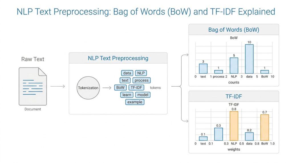
Now we can look at the classic bag-of-words idea. In this representation, each document becomes a row, each token becomes a column, and each cell stores how often that token appears in that document. The model ignores word order, which is a trade-off: we lose some nuance, but we gain a simple, sturdy numeric table that machine learning algorithms understand well. Scikit-learn also lets us add n-grams, which are token sequences of length n; for example, bigrams are two-word chunks that help preserve a little local context, so phrases like “is this” can carry more meaning than single words alone.
TF-IDF builds on that same table, but it adds a sense of proportion. Term frequency tells us how often a term appears in one document, while inverse document frequency lowers the weight of terms that appear in many documents across the whole corpus, which means a word that shows up everywhere gets less attention than a word that helps distinguish one document from another. In scikit-learn, TfidfVectorizer combines the counting and weighting steps into one tool, and it can even smooth the weighting to avoid divide-by-zero problems. This is why TF-IDF often feels like a smarter version of bag of words: it still counts words, but it listens more carefully to the ones that actually separate documents.
As we keep walking, it helps to remember that preprocessing is not a fixed ceremony. Scikit-learn lets you customize the preprocessor, tokenizer, and analyzer; the preprocessor transforms the whole document, the tokenizer splits it into tokens, and the analyzer can replace both when you need full control. That flexibility matters when you have HTML to strip, special token rules to enforce, or text that needs stemming or lemmatization, which are techniques for reducing words to a simpler base form. The cleanest workflow is the one that matches your data, because the best text preprocessing basics are the ones that make your text look ordinary enough for a model to learn from it.
Tokenization and Stop Words (scikit-learn.org)
Now that we have the broad idea of turning text into numbers, we arrive at the gatekeepers: tokenization and stop words. This is the stage where scikit-learn decides which pieces of language become features and which pieces stay in the background. Think of it like sorting a bag of mixed puzzle pieces before we start building the picture. The tokenizer chops the document into tokens, while stop words remove common words that often carry little signal for prediction. In scikit-learn, this work happens inside the analyzer pipeline, so one pass can handle preprocessing, tokenization, and n-gram creation. If we skip this step or handle it carelessly, the model can end up staring at a noisy pile of words instead of a useful pattern.
If you’ve ever wondered, “How does tokenization work in scikit-learn?” the default behavior is a little more disciplined than everyday reading. The standard word tokenizer lowercases text, treats punctuation as a separator, and keeps tokens made of two or more alphanumeric characters. That means “Hello, world!” and “hello world” land in the same bucket, while tiny fragments like a lone comma or a single letter usually never become features. In other words, tokenization is not trying to preserve every character; it is trying to produce a stable set of word-like pieces that a model can count reliably. This is one reason bag of words and TF-IDF stay manageable: the vocabulary focuses on consistent tokens instead of stray punctuation and scraps.
Stop words enter next, and this is where the story gets a little more subtle. Words such as “and,” “the,” and “him” often appear so frequently that they blur the signal we actually care about, so removing them can make a text model cleaner and easier to train. But scikit-learn also warns us that its built-in English list is not a universal answer, because a word that looks boring in one task can be valuable in another, like style or personality analysis. A list that is too aggressive can erase useful clues, while a list that is too small can leave the model swimming in filler. Just as important, the stop-word list must go through the same preprocessing and tokenization as the text itself, or we can accidentally keep half a word and remove the other half.
That mismatch is the trap many beginners run into. What happens when stop words and tokenization do not agree? Scikit-learn gives the classic example of “we’ve,” which the default tokenizer splits into “we” and “ve”; if your stop list contains “we’ve” but not “ve,” the leftover fragment can survive in the final matrix. This is why the docs treat stop-word handling as a matching game rather than a separate cleanup step. Think of it like labeling storage bins after sorting the objects: if the labels do not match the pieces, the wrong things stay on the shelf. When your data needs special rules, you can replace the tokenizer or even the whole analyzer, and scikit-learn leaves room for custom logic such as pretokenized text, lemmatization, or other domain-specific filtering.
When we put the pieces together, the practical lesson is simple: choose tokenization and stop-word rules that fit the job, not the other way around. If a corpus has its own noisy high-frequency terms, scikit-learn can also use max_df to drop words that appear in too many documents, which acts like a corpus-specific stop-word filter. That can be a gentler option than hard-coding a list, especially when we are still learning what the text really contains. If you are unsure where to begin, start with the default tokenizer, inspect the vocabulary it produces, and then tune the stop-word strategy from there. In practice, the best setup is the one that keeps meaningful distinctions while trimming away the language that only fills space.
Building Bag of Words (scikit-learn.org)
So how do we build a bag of words in scikit-learn when the text still feels messy? We hand the corpus to CountVectorizer, the tool that learns a vocabulary and turns raw documents into a document-term matrix. In that matrix, each row is a document and each column is a token, so the model sees counts instead of sentences. Scikit-learn’s guide describes this as tokenizing the text, assigning an integer id to each token, and counting how often those tokens appear in each document.
The usual move is fit_transform, because it learns and counts in one pass. fit builds the vocabulary dictionary from the training corpus, transform reuses that learned vocabulary on new text, and fit_transform is the more efficient shortcut that does both together. Once the vectorizer has seen your corpus, get_feature_names_out() shows the learned column names, while vocabulary_ stores the mapping from terms to feature indices. That is the quiet moment where text starts to become a table.
A tiny example makes the shape easier to picture. If one document says “This is the first document” and another says “This is the second second document,” the vectorizer creates one row per document and places counts only where words appear. Scikit-learn notes that most text corpora use only a very small slice of a large vocabulary, so the resulting matrix is usually more than 99% zeros. That is why bag-of-words output is typically stored as a sparse matrix, which saves memory and keeps the arithmetic fast.
This is where tuning starts to feel like adjusting a camera lens. ngram_range=(1, 2) tells CountVectorizer to keep both single words and two-word phrases, which can preserve a little local context without abandoning the bag of words idea. The default word pattern keeps tokens with two or more alphanumeric characters and treats punctuation as a separator, while max_df, min_df, and max_features let you trim tokens that are too common, too rare, or simply too many. In practice, this is how we stop the vocabulary from growing wild before it reaches the model.
If you have ever asked, “Why does my bag of words look noisier than I expected?” the answer is usually that the vocabulary needs a little housecleaning. CountVectorizer lets you lowercase text, remove accents, override the preprocessor, tokenizer, or analyzer, and supply your own stop-word list; the scikit-learn docs also warn that the built-in English stop-word list is not a universal solution. max_df can work like a corpus-specific stop-word filter, and the vectorizer will only use the vocabulary it learned from training when it transforms later documents. That makes the workflow predictable: learn once, reuse many times.
Once the matrix exists, the story shifts from language to shape. We no longer carry whole sentences into the model, only numbers that mark which words appeared and how often, and that is enough for many linear classifiers and clustering methods to start finding patterns. Scikit-learn’s text guide points out that bag of words works well with document classification, clustering, and topic discovery, even though it deliberately ignores most of the document’s internal structure. That trade-off is the heart of the method: we lose order, but we gain a clean bridge from messy text to machine-learning input.
Understanding TF-IDF Weights (scikit-learn.org)
When we move from simple word counts to TF-IDF, the story changes from “how often did this word appear?” to “how useful is this word for telling documents apart?” That shift is the heart of TF-IDF weights. In scikit-learn, TfidfVectorizer builds those weights for us by turning raw documents into a matrix of TF-IDF features, and it does so by combining the counting step with the weighting step in one tool.
The easiest way to picture this is to imagine a classroom where everyone keeps saying the same polite filler words. Those words may be present in almost every notebook, but they do not help us identify who wrote what. TF-IDF, which stands for term frequency–inverse document frequency, gives a word more weight when it appears often in one document but less weight when it appears everywhere in the collection. Scikit-learn’s docs describe this as scaling down the impact of tokens that occur very frequently across the corpus because those tokens are usually less informative.
So what are the two pieces doing? Term frequency is the local part: it measures how often a term appears inside a single document. Inverse document frequency is the broader part: it checks how many documents in the whole set contain that term, then lowers the score for words that show up in many places. In the default formulation, scikit-learn computes TF-IDF as term frequency multiplied by inverse document frequency, and when smooth_idf=True, it adds a small correction that prevents zero divisions by behaving as though one extra document contained every term once.
That smoothing detail matters because it keeps the math steady even when the corpus is small or lopsided. Scikit-learn also offers sublinear_tf=True, which replaces raw term frequency with 1 + log(tf), so a word appearing 20 times does not become 20 times more important than a word appearing once. On top of that, norm='l2' makes each output row have unit length, which means the vector behaves nicely when we compare documents using cosine similarity, a measure of how closely two directions in space point the same way.
If you are wondering, “How does TfidfVectorizer work in scikit-learn?” the answer is that it learns vocabulary and IDF values during fit, then reuses them during transform. The class is equivalent to CountVectorizer followed by TfidfTransformer, which is a helpful mental model because it reminds us that TF-IDF is not magic; it is counting first and reweighting second. The resulting matrix is sparse, meaning most entries are zeros, because each document only uses a tiny slice of the full vocabulary.
That sparse matrix is where the intuition becomes practical. A word that appears in almost every document, like a generic filler term, ends up with a smaller TF-IDF weight, while a word that helps separate one document from another gets a stronger voice. In other words, TF-IDF weights do not erase common words; they quietly step them back so the more distinctive words can speak louder. Scikit-learn’s implementation even exposes the learned idf_ vector, so you can inspect which terms the model considered broadly common across the corpus.
The real payoff is that this weighting makes text feel a little less noisy for downstream models. Instead of treating every repeated word as equally meaningful, TfidfVectorizer gives us a matrix where repetition, rarity, and document-level context all work together. That is why TF-IDF often feels like a more thoughtful version of bag of words: it still keeps the simple table structure, but it adds a sense of emphasis, and that extra emphasis is often what helps a model notice the words that actually carry the story.
BoW vs TF-IDF Comparison (scikit-learn.org)
Now that we have seen how text becomes counts and then weights, the BoW vs TF-IDF comparison starts to feel less like a technical split and more like two different ways of listening to the same conversation. Bag of words, or BoW, hears every word as a tally mark; TF-IDF hears the same words but asks which ones actually help tell documents apart. If you are wondering, “Which one should I use for text classification?”, that is the right question to ask, because the answer depends on whether you want simplicity or selectivity. In scikit-learn, this choice often comes down to CountVectorizer for bag of words and TfidfVectorizer for TF-IDF.
Bag of words is the more literal reader of the two. It keeps the vocabulary straightforward: each term gets counted, and every repeated appearance pushes the number higher, whether the word is rare or common. That makes BoW easy to explain, easy to inspect, and often surprisingly effective when your model only needs to know that a word appeared at all. The trade-off is that common words can dominate the picture, so a document filled with generic language may look more important than it really is.
TF-IDF steps in when those raw counts start to blur the signal. It still begins with the same document-term matrix, but it lowers the weight of words that appear everywhere and lifts words that are more distinctive within the corpus. Think of it like a group photo: BoW gives every face the same visual space, while TF-IDF quietly highlights the people who make this photo different from every other one. That is why TF-IDF often works better when documents share a lot of background language but differ in a few key details.
The practical difference becomes clearer when we look at what each representation rewards. BoW rewards repetition inside a document, so a word that appears ten times gets ten counts, full stop. TF-IDF rewards repetition only when it is meaningful, which means a word that appears often in one document but rarely elsewhere gets a stronger signal than a word that shows up in every other document too. In other words, bag of words answers, “What is here?” while TF-IDF leans toward, “What is here that helps identify this text?”
That difference matters a lot when we build models from real-world text. For tasks like spam detection, topic classification, or sentiment analysis, TF-IDF often gives linear models a cleaner starting point because it downplays filler and emphasizes discriminative terms. BoW can still do very well, especially with enough data or with n-grams that capture short phrases, but it may need extra help from stop-word removal or frequency thresholds to stay focused. So the choice is not about one method being right and the other being wrong; it is about matching the representation to the kind of signal you expect.
There is also a small but important intuition about noise. BoW treats every counted word as equally trustworthy, which can be useful when raw frequency itself carries meaning, such as in short documents or controlled vocabulary tasks. TF-IDF adds a layer of caution, assuming that some words are too common to be very informative and should therefore speak more softly. That extra caution can make the feature space feel more balanced, especially when the corpus has lots of shared terminology.
In scikit-learn, that difference is easy to test because the tools sit so close together. CountVectorizer gives you the counts first, and TfidfVectorizer wraps the same general process with TF-IDF weighting on top, so you can compare them without changing the rest of your workflow. A useful habit is to start with bag of words when you want a simple baseline, then try TF-IDF when the vocabulary looks crowded or when common terms seem to drown out the useful ones. That way, you are not choosing a theory in the abstract; you are choosing the representation that lets your model hear the text more clearly.
Python Example with Scikit-Learn (scikit-learn.org)
When we first turn a few sentences into features, the hardest part is often believing that a tiny snippet of Python can produce something a model can read. CountVectorizer is the starting point for bag of words: it learns a vocabulary from the training text, then turns each document into a sparse document-term matrix of token counts. TfidfVectorizer takes the same idea one step further and produces TF-IDF features, which is why it is described in scikit-learn as equivalent to CountVectorizer followed by TfidfTransformer.
from sklearn.feature_extraction.text import CountVectorizer, TfidfVectorizer

corpus = [
    "The cat sat on the mat",
    "The dog sat on the log",
    "The cat chased the dog"
]

count_vec = CountVectorizer()
X_counts = count_vec.fit_transform(corpus)

print(count_vec.get_feature_names_out())
print(X_counts.toarray())

tfidf_vec = TfidfVectorizer()
X_tfidf = tfidf_vec.fit_transform(corpus)

print(tfidf_vec.get_feature_names_out())
print(X_tfidf.toarray())
This example shows the full journey in miniature: fit_transform learns the vocabulary and returns the matrix in one pass, get_feature_names_out() reveals the learned columns, and the output stays sparse behind the scenes because most text corpora use only a small fraction of their vocabulary in any one document. That sparse design matters because it keeps the matrix compact even when the vocabulary grows.
If you look at the bag-of-words output first, you will see plain counts: every time a token appears, its column ticks upward. That is the whole promise of BoW, and it is surprisingly powerful because it gives us a stable table of numbers without asking the model to understand word order. In scikit-learn, the default word tokenizer also lowercases text, ignores punctuation as a separator, and keeps tokens made of two or more alphanumeric characters, so the vocabulary stays consistent across documents. If you want to reduce noise further, max_df can drop terms that appear in too many documents, acting like a corpus-specific stop-word filter.
TF-IDF adds a little more judgment to the same table. Instead of treating every repeated word as equally useful, it downweights terms that appear everywhere and upweights terms that help distinguish one document from another. Scikit-learn defines TF-IDF as term frequency multiplied by inverse document frequency, with optional smoothing to avoid zero divisions, and the default norm='l2' makes each row unit length so cosine-style comparisons behave well. This is why TF-IDF often feels like bag of words with better ears: it still counts words, but it listens more carefully to the ones that matter.
Here is the practical choice we usually make in a real project. If you want the clearest baseline, start with CountVectorizer and inspect the vocabulary it builds. If the text has a lot of shared filler language, move to TfidfVectorizer, which wraps the counting and weighting steps into one cleaner pipeline and often gives linear models a more balanced input space. In both cases, the workflow stays the same: learn on training text, reuse the learned mapping on new text, and let the matrix do the talking. That is the quiet trick behind a good Python example with scikit-learn: once the text becomes counts or TF-IDF weights, the model can finally start spotting patterns.