Window Function Basics
If you have already spent time with SELECT, WHERE, and GROUP BY, you may have felt the first little crack in the wall: you can summarize data, but you lose the row-by-row story. That is where SQL window functions step in. They let us calculate totals, rankings, and comparisons without collapsing the table into a single summary row, which makes them perfect for analytics work. Think of them as a way to look at each row through a moving pane of glass, where the row stays visible and the calculation travels with it.
The heart of a window function is the OVER clause, which tells SQL what neighborhood to use for the calculation. A window is the set of rows a function can see at one time, and that set can be the whole table, a grouped slice of the table, or even a tiny moving range around the current row. This is the first idea to hold onto: unlike regular aggregate functions, which usually reduce many rows into one, window functions return a result for every row. That difference is what makes them feel so useful once you see them in action.
Here is the question many people ask when they first meet them: how do SQL window functions work without changing the shape of the result? The answer is that the query keeps each original row, then adds a calculated column beside it. We can say, “Give me the rank of each sale within its store,” or “Show me a running total of revenue over time,” and SQL will do that while preserving the full detail. In other words, window functions let us layer analysis on top of the data instead of flattening the data first.
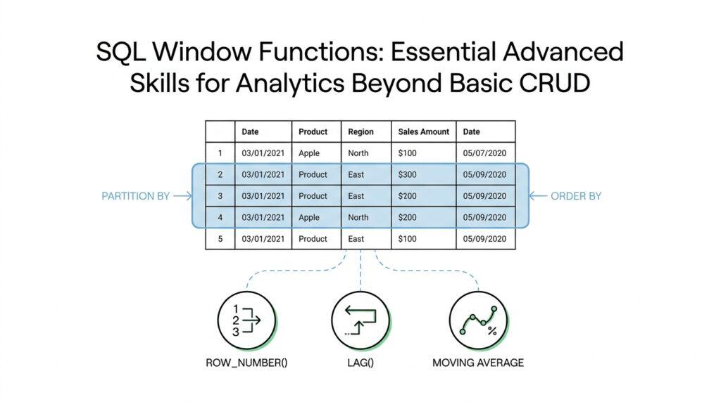
To make that possible, we usually define two more pieces of the window: PARTITION BY and ORDER BY. PARTITION BY means “split the rows into separate buckets,” like putting all sales from each store into their own stack. ORDER BY means “arrange the rows inside each bucket,” which is important when the calculation depends on sequence, such as ranking or running totals. Once those two pieces are in place, the function knows both the group it belongs to and the order it should follow.
It helps to picture a classroom. PARTITION BY separates students into different classrooms, ORDER BY lines them up inside each classroom, and the window function asks a question about each student while still keeping every student in view. If we want a running sum, the function starts at the first row in the ordered partition and adds values as it moves forward. If we want a rank, it compares the current row with the others in the same partition and assigns a position. This is why SQL window functions are so powerful for analytics: they can compare, accumulate, and measure without losing context.
There is one more small but important idea: the frame. A frame is the exact slice of rows used for a calculation around the current row, and it becomes especially important for moving calculations like rolling averages. You do not need to master every frame rule at once, but it helps to know that the window is not always the same as the full partition. Sometimes the function looks at all rows in the partition, and sometimes it looks only at the rows immediately before and after the current one. That fine-grained control is what turns window functions from a neat trick into a serious analytical tool.
Once these pieces click, the pattern becomes easier to read and easier to write. You choose a window function, decide how to split the data with PARTITION BY, decide how to line it up with ORDER BY, and then let the OVER clause carry the logic. From there, the door opens to rankings, running totals, moving averages, and other patterns that would be awkward or repetitive with basic SQL alone. And now that the basics are in place, we can start using SQL window functions to solve the kinds of questions analysts ask every day.
Understanding OVER Clause
When you start reading SQL window functions, the OVER clause is the part that makes the whole sentence make sense. It acts like an address label for the calculation, telling SQL where to look while still keeping every original row in place. That is why a window function can add analysis beside the data instead of replacing the data with a single summary row.
The shape is familiar once you see it: a function name, then OVER, then the rules for how that function should travel through the result set. In PostgreSQL’s documentation, the OVER clause is what turns an ordinary aggregate like avg into a window function, and SQL Server documents the same idea for analytic and ranking functions. If you have ever asked, “How does SQL calculate a rank without collapsing my rows?”, the answer lives right here.
The first helper inside OVER is PARTITION BY, and it works like drawing boundaries on a map. Instead of letting every row talk to every other row, it splits the result set into separate partitions, so each row is measured against the rows in its own group. If you leave PARTITION BY out, the window can cover the whole table, which is why a running total or overall average can be computed once and repeated alongside each row.
The next helper is ORDER BY, and this is where the story gains movement. ORDER BY inside OVER tells SQL the sequence to follow while it processes the rows in each partition, but it does not have to match the final display order of the query output. That distinction matters because ranking and running calculations depend on sequence, not just membership, so the order inside the window can change the answer even when the visible table looks the same.
Here is where the idea gets a little more delicate, and that is perfectly normal. The OVER clause can also include a frame, which is the exact slice of rows a function uses around the current row, and PostgreSQL notes that some functions such as first_value, last_value, and nth_value pay attention to that frame rather than the whole partition. That is why a running sum behaves like a moving tally: the window function looks backward through the frame as it advances one row at a time.
This is also why the same function can feel different depending on the OVER clause you give it. An aggregate used as a window function will compute across the current window frame, so avg(salary) OVER (PARTITION BY depname) describes one kind of answer, while adding ORDER BY can turn the same idea into a progressive calculation instead of a whole-partition result. In other words, the function name tells us what math to do, and the OVER clause tells us how far that math should reach.
Once you begin reading OVER this way, it stops looking like syntax decoration and starts feeling like the control panel for SQL window functions. We choose the partition, choose the order, and, when needed, narrow the frame, then SQL carries that logic row by row without losing the larger picture. That is the mental model that makes the next examples much easier to follow.
Partitioning Result Sets
Now that we have the OVER clause in view, the next question is how to make the calculation feel local instead of global. Partitioning result sets is where SQL window functions start behaving like a careful analyst at a desk, not a machine staring at the whole table at once. You ask, “What does PARTITION BY do in SQL window functions?” and the answer is that it breaks one big result set into smaller, meaningful neighborhoods while keeping every row visible.
That idea matters because analytics often lives in comparisons within a category, not across everything at once. Imagine a sales table with rows from many stores, and you want to know each sale’s rank inside its own store. If we used the full table as one window, a small neighborhood store would be measured against the busiest location in the company, which would blur the story. With partitioning, each store gets its own lane, and the calculation stays fair and focused.
This is the first place where PARTITION BY feels different from GROUP BY. GROUP BY is like folding a pile of papers into a single summary sheet, while PARTITION BY is like placing the papers into labeled trays and then reading them one by one. The rows do not disappear, and that is the key advantage of SQL window functions. We can still see the original sale, order, or signup, and we can still attach a comparison that belongs to that exact row.
A partition can be as broad or as narrow as the question demands. If you partition by store_id, every store gets its own result set slice; if you partition by store_id and month, you create smaller pockets that let you study each store over time. In practice, this is how we build store-specific rankings, department-specific averages, or customer-specific running totals without writing separate queries for every category. The partition becomes the frame of reference, and the function does its work inside that frame.
This is also where many beginners have a useful little breakthrough. Partitioning does not change the data itself; it changes the audience the calculation is speaking to. A moving average over one partition can tell a story about a single product line, while the same function over another partition can reveal a very different pattern in another region. Once you see that, SQL window functions stop feeling like abstract syntax and start feeling like tools for shaping perspective.
There is a practical habit worth building here: choose the partition based on the question, not the table. If you are asking about performance inside each team, partition by team. If you are asking about behavior inside each month, partition by month. The wrong partition can make a result look technically correct but analytically misleading, which is why this step deserves attention before we ever look at the numbers.
So when we talk about partitioning result sets, we are really talking about setting boundaries around meaning. We keep the full row detail, but we tell SQL which rows should compare with one another, and that choice gives rankings, percentages, and running totals their context. That small decision is what lets SQL window functions move from broad summaries to precise, human-shaped analysis.
Ordering and Window Frames
At this point in our journey, the data has already been divided into meaningful partitions, but it still needs a sense of direction. That is where ORDER BY inside OVER steps in: it tells SQL how to walk through the rows inside each partition, and that order can be different from the final sort order of the query output. If you have ever wondered, “Why does my running total change when I add ORDER BY to a SQL window function?”, this is the reason. The order inside the window is part of the calculation itself, not just the display.
Once the rows have an internal order, functions like row_number start acting like a line leader. PostgreSQL notes that row_number assigns sequential numbers within each partition according to the ORDER BY clause, and tied rows are numbered in an unspecified order unless you add more columns to break the tie. That tie behavior matters because window function rows that are not distinct on the ORDER BY columns are called peers, and several ranking functions give the same answer to every row in a peer group. In plain language, if two rows look identical to the window’s sort rule, SQL treats them like neighbors standing shoulder to shoulder.
Now we meet the part that often feels mysterious at first: the window frame. A window frame is the exact slice of rows a function can see around the current row, which is narrower than the whole partition for some calculations. Think of it like the bright circle from a flashlight: the partition is the whole room, but the frame is the area currently lit. Some window functions read only that lit area, while others care about the entire partition, so the frame quietly changes the meaning of the result.
The default frame is the detail that explains many surprises. When ORDER BY appears in OVER, PostgreSQL says the frame runs from the start of the partition through the current row, plus any rows that tie with it on the ORDER BY columns; when ORDER BY is omitted, the default frame is the whole partition. That is why sum(salary) OVER (ORDER BY salary) behaves like a running total instead of a full-partition total. The calculation is not counting everything at once; it is stepping forward row by row and remembering what it has already passed.
This is also the reason some functions deserve extra caution. PostgreSQL documents that first_value, last_value, and nth_value look only at the window frame, not automatically at the whole partition, and the default frame can make last_value feel unintuitive because it stops at the current row’s peer group. In other words, if you expected “last row in the department” but the frame only reaches the current peer, you may get a much smaller answer than you wanted. That is not a bug in the logic; it is the frame doing exactly what you asked, even if the request was a little too narrow.
When you do want a whole-partition result, you have a few clear options. You can omit ORDER BY so the frame expands to the full partition, or you can spell out a frame like ROWS BETWEEN UNBOUNDED PRECEDING AND UNBOUNDED FOLLOWING to cover every row in the partition. PostgreSQL also supports different frame units such as RANGE, ROWS, and GROUPS, which let you choose whether the frame follows physical rows, sort-value ranges, or peer groups. That gives SQL window functions a surprising amount of precision, almost like choosing between a wide brush and a fine pen.
So when you read a window function now, you can ask three questions in order: what rows belong to the partition, how are those rows ordered, and how far does the frame reach from the current row. That mental checklist turns ORDER BY and window frames from syntax into a story you can follow. First we set the neighborhood, then we set the walking path, and finally we decide how much of the path each row gets to see. With that picture in place, the next examples feel less like magic and more like a carefully arranged walkthrough.
Ranking and Percentiles
When ranking and percentiles enter the picture, SQL starts answering the question behind the numbers instead of merely listing them. If we have ten orders, ten employees, or ten test scores, we often want to know who came first, who tied, and where each row sits in the crowd. Window ranking functions do that without collapsing the rows, and PostgreSQL requires them to be used with OVER, which keeps each record visible while adding the comparison beside it.
The first three ranking tools feel like cousins with slightly different habits. row_number() gives every row a unique position, even when two rows look the same to the sort order; rank() gives tied rows the same position but leaves gaps afterward; and dense_rank() also gives tied rows the same position, but it does not leave gaps. PostgreSQL defines peers as rows that are not distinct on the ORDER BY columns, and these ranking functions return the same answer for every row in a peer group.
That difference matters because it changes the story the data tells. Imagine two employees tied for second place: with rank(), the next person becomes fourth, because the shared second place creates a gap; with dense_rank(), the next person becomes third, because the sequence stays compact. When you are reading ranking and percentiles in SQL, rank() is often the right choice when the tie itself should be visible, while dense_rank() feels better when you want a tidy list of levels rather than skipped numbers.
Once the basic ranking feels comfortable, percent-based functions answer the quieter question: how far through the list is this row? percent_rank() returns a relative rank from 0 to 1 using the formula (rank - 1) / (total partition rows - 1), so it tells you how far a row stands from the bottom of its partition. cume_dist() goes a step farther and reports the fraction of rows that come before the current row or belong to its peer group, which also ranges from 1/N to 1. In everyday language, percent_rank() says “where does this row land on the ladder,” while cume_dist() says “what share of the group is at or below this row.”
If you want to split data into rough buckets, ntile() gives you another useful lens. PostgreSQL defines it as an integer from 1 to the number of buckets you ask for, dividing the partition as evenly as possible. That makes it handy for quartiles, deciles, and other broad groupings, but it is not the same thing as a true percentile value; it is more like placing books onto equal shelves than measuring the exact height of each book.
The exact percentile story uses a slightly different tool: ordered-set aggregates such as percentile_cont() and percentile_disc(), which use WITHIN GROUP (ORDER BY ...) rather than OVER. PostgreSQL describes percentile_cont() as a continuous percentile that interpolates between adjacent values when needed, while percentile_disc() returns the first value whose position in the ordering equals or exceeds the requested fraction. That means percentiles are not always window functions in the strict sense, but they belong in the same analytical family because they help us locate a value inside an ordered distribution.
So when we choose among ranking and percentiles, we are really choosing the question we want answered. If we want an exact seat in line, we reach for row_number(), rank(), or dense_rank(); if we want a relative standing, we use percent_rank() or cume_dist(); if we want broad buckets, ntile() gives us a practical map; and if we want the median or the 90th percentile value itself, percentile_cont() or percentile_disc() can do the measuring. Once that distinction clicks, the rest of analytics feels much easier to read, because every function is now telling a different part of the same story.
Running Totals and Moving Averages
Now that we have partitions, order, and frames in place, we can start using SQL window functions for the two patterns analysts reach for most often: running totals and moving averages. These are the calculations that let you watch a number grow over time instead of staring at one isolated summary. A running total is a cumulative sum, which means each row carries the total of itself plus everything that came before it in the chosen order.
That sounds abstract until you picture a sales dashboard. On Monday, revenue might look small; by Friday, we want to see the whole week’s buildup, not just the final number. A running total gives us that trail, row by row, so we can follow momentum as it forms. Because we already know how ORDER BY shapes the path through the partition, the key idea here is that the calculation remembers every earlier step.
Here is the kind of query shape that makes that happen:
SUM(amount) OVER (
  PARTITION BY store_id
  ORDER BY sale_date
  ROWS BETWEEN UNBOUNDED PRECEDING AND CURRENT ROW
) AS running_revenue
This is a classic SQL window function pattern. SUM(amount) does the math, PARTITION BY store_id keeps each store in its own lane, and the frame from the first row through the current row tells SQL to keep adding as it moves forward. The result is not one grand store total; it is a live total attached to each sale, which makes trends much easier to read.
Once we have that cumulative picture, the next question is often whether the raw ups and downs are hiding the real story. That is where a moving average comes in, sometimes called a rolling average. Instead of adding everything from the start, a moving average looks at a small window of recent rows and smooths out the noise, like stepping back from a jittery graph so the larger shape becomes visible.
This is especially useful when daily data bounces around. A single spike in orders or a quiet afternoon can make a chart look dramatic, even when the underlying trend is steady. By averaging only the most recent rows, we get a softer, more readable signal. In SQL window functions, that usually means choosing a frame like “the current row and the two rows before it,” which creates a three-row moving average.
AVG(amount) OVER (
  PARTITION BY store_id
  ORDER BY sale_date
  ROWS BETWEEN 2 PRECEDING AND CURRENT ROW
) AS moving_avg_3_days
The important part is the frame. ROWS BETWEEN 2 PRECEDING AND CURRENT ROW tells SQL to look at a sliding slice of three rows at a time, not the whole history. That means each new row pushes the window forward, dropping the oldest row and bringing in the newest one. If you are asking, “How do I calculate a moving average in SQL without losing the row detail?”, this is the pattern we reach for.
Running totals and moving averages solve different kinds of questions, and that difference matters. A running total answers, “How much have we accumulated so far?” while a moving average answers, “What does the recent trend look like right now?” One emphasizes growth, the other emphasizes smoothing. Both belong to the same family of SQL window functions, but they tell us different parts of the same story.
There is one small habit that saves a lot of confusion: always check what your frame is doing before you trust the result. If you use ROWS, you are counting physical rows; if your data has gaps in dates, that may be exactly what you want, or it may mean you need a different approach. We do not need to fear that detail, but we do need to notice it, because a moving average over sparse data can tell a very different story from one over evenly spaced rows.
The safest way to work is to build the calculation in layers. First, confirm the partition gives you the right group. Then, make sure the order matches the timeline you care about. Finally, choose a frame that matches the question you are asking, and the running total or moving average will do the rest. Once that pattern feels familiar, we can start mixing these calculations with other analytical tools and get even more from the same table.