Overview of LLMs
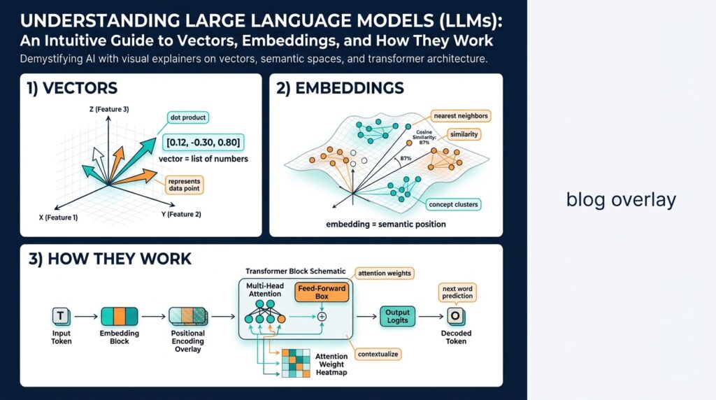
Large Language Models (LLMs) have become the backbone for tasks ranging from code completion to customer-support automation, and understanding their core mechanics—transformer architecture, tokenization, embeddings, and vectors—lets you make pragmatic design choices. In practice, an LLM is a statistical model that maps discrete tokens into continuous vector spaces and learns patterns across massive text corpora; those learned vector representations (embeddings) are what power semantic similarity, retrieval, and downstream reasoning. We’ll treat the model as both a probabilistic predictor and a vector factory: you care about it for generation, and you care about its embeddings for search and retrieval-augmented workflows.
At the heart of modern LLMs lies the transformer, an architecture built around self-attention that lets the model weigh relationships between tokens regardless of distance in the input. Tokenization converts raw text into subword units or tokens, which the model embeds into vectors before applying multi-head attention and feed-forward layers; attention scores tell the model which tokens to emphasize when predicting the next token. Because attention operates on token-level vectors, the same mechanism that enables fluent generation also produces contextual embeddings you can extract and reuse. When you design a system, recognizing this dual role helps you decide whether you need full-sequence decoding or just the vector outputs.
Training and fine-tuning are where behavior emerges: during pretraining, the objective is typically next-token prediction or masked token reconstruction, which encourages the model to internalize syntax, semantics, and world knowledge. Fine-tuning on domain data or using supervised objectives aligns the LLM with specific tasks like intent classification or summarization; reinforcement learning from human feedback (RLHF) can further shape preferences such as helpfulness or safety. Larger models and more diverse datasets generally improve capabilities, but returns diminish and costs rise—so weigh parameter scale against latency, cost, and deployment complexity when you choose a model for production.
Embeddings are the bridge from language to structured tooling: they map phrases, sentences, or documents into vectors in high-dimensional space where geometric proximity implies semantic similarity. You use vector operations—cosine similarity or Euclidean distance—to implement semantic search, document clustering, or nearest-neighbor retrieval for retrieval-augmented generation (RAG). How do you choose embedding dimensionality for your use case? Test different dimensions and measure downstream retrieval precision and latency: higher dimensions can capture nuance but increase storage and compute for nearest-neighbor searches, so balance representation quality with operational constraints.
When you run inference, decoding strategy matters: greedy decoding, beam search, top-k, and nucleus (top-p) sampling each trade off between determinism and diversity. Temperature controls output randomness; a lower temperature yields conservative, high-probability continuations while a higher temperature produces varied and creative text. For production features like email drafting or policy generation, we prefer deterministic settings with safety filters; for exploratory or creative tools, you can tune temperature and sampling to encourage novelty. Also consider response length, stop tokens, and prompt engineering—small prompt changes can produce large behavioral differences.
Operationalizing LLMs and vectors introduces engineering considerations beyond model selection: quantization and pruning reduce memory and inference costs, while vector databases and approximate nearest neighbor (ANN) indexes (HNSW, IVF, PQ) speed up retrieval at scale. You’ll need to design pipelines for embedding generation, index maintenance, and consistency between your retrieval layer and the model used to generate embeddings. Monitor latency tail, throughput, and embedding drift as the underlying data evolves; automated reindexing and versioned feature stores help maintain retrieval quality as you iterate.
We must also confront limitations: hallucinations, calibration errors, and biases are persistent risks that affect trust and correctness. Evaluate models using both automated metrics and human review, deploy guardrails like factuality checks or external retrieval, and keep a human-in-the-loop for high-risk outputs. Logging, changelogs for model versions, and post-deployment A/B testing let you measure real-world impact and decide whether to fine-tune, change prompts, or swap models.
Building on these ideas, we’ll next dive deeper into how embeddings are computed, compared, and indexed—walking through code examples for generating vectors, tuning dimensionality, and integrating an ANN index so you can deploy scalable semantic search and RAG pipelines.
Tokenization Basics
Building on this foundation, tokenization is the discrete step that turns raw text into the atomic units an LLM understands: tokens. Tokenization (the process of splitting text into tokens) and the specific token vocabulary you choose shape sequence length, model cost, and how semantics are preserved before any embeddings are computed. You’ll see effects everywhere—from how many model tokens a user prompt consumes to whether domain-specific terms remain intact or get fragmented. Understanding tokenization fundamentals helps you control latency, storage, and the fidelity of semantic search when we later convert tokens into vectors.
At its core, tokenization strategies fall into a few families: character-level, word-level, and subword-level tokenizers. Subword tokenization (we’ll define this as splitting words into smaller, reusable units) is the dominant approach because it balances vocabulary size and coverage; algorithms such as byte-pair encoding (BPE) and unigram language modeling (used in SentencePiece) produce subword units that capture frequent morphemes or byte sequences. Byte-level tokenizers operate on raw bytes, avoiding Unicode normalization pitfalls and ensuring deterministic encoding across languages, while word-level tokenizers keep whole words intact but explode the vocabulary. Each approach has trade-offs: smaller vocabularies reduce model parameters, but aggressive splitting increases token counts and can harm latency.
Practical tokenization behavior often surprises engineers, so inspect examples on your data. For instance, a BPE-style tokenizer might split “unbelievable” into [“un”, “believ”, “able”] and map them to IDs like [1024, 3456, 78]. Here’s a short conceptual snippet showing how you’d check tokenization with a tokenizer object in Python:
# pseudo-code
ids = tokenizer.encode("def fetch_data():")
print(ids)        # e.g., [134, 879, 23, 11]
print(tokenizer.decode(ids))
Run this on representative prompts to measure average tokens-per-request; that metric directly affects inference cost and context utilization. Also verify that the tokenizer used to generate embeddings matches the one used by the model that will later consume those embeddings—mismatches cause token alignment issues, truncation differences, and degraded retrieval relevance.
Why does this matter for embeddings and retrieval? Because embeddings are computed per token (or per pooled token representation) and geometric similarity depends on how text is sliced. If a frequent compound term in your domain splits into many rare subwords, its embedding may be diffused across multiple vectors, reducing nearest-neighbor accuracy. Likewise, tokenization defines the effective context window: a 4,096-token model can handle fewer English words if your tokenizer splits aggressively. So when you plan a retrieval-augmented generation (RAG) pipeline, measure both tokens-per-document and the vector dimensionality trade-offs to balance precision and storage.
Beware of tokenization pitfalls: normalization choices (lowercasing, accent stripping), special-token handling (padding, BOS/EOS), and how emojis or code are split can introduce bias or break prompts. How do you decide when to add custom tokens? Add tokens when a frequent, semantically cohesive unit in your corpus is split in ways that dilute meaning—examples include product SKUs, API names, or multi-word technical identifiers. Adding a few hundred targeted tokens typically yields better retrieval and generation than wholesale vocabulary changes.
As a rule, test tokenization on realistic inputs, collect token-length histograms, and run a small A/B comparing retrieval or generation quality with and without custom tokens. For code-heavy products, include language-specific tokens; for multilingual systems, prefer byte-level or SentencePiece-style tokenizers. These practical checks ensure that when we move from tokens to embeddings, the vectors you index preserve the semantic structure you care about. Next, we’ll look at how those token-level representations are converted into the continuous vectors you use for search and downstream tasks.
Vectors and Embeddings
When you move from discrete text to numerical reasoning, two concepts become the workhorses: vectors and embeddings. These dense numeric encodings let models and retrieval systems reason about meaning geometrically, so you can implement semantic search, clustering, and similarity-based routing with distance computations rather than brittle string matching. Because we’ll rely on these representations in downstream pipelines, understanding their geometry and practical trade-offs early saves a lot of rework later.
A dense representation maps text, phrases, or documents into points in high-dimensional space where proximity implies related meaning. In that space, nearest-neighbor queries and distance metrics capture semantic relationships that keyword queries miss, which is why retrieval-augmented generation and context selection use these encodings for relevance. We’ll treat the geometry as intentional: angles indicate directionality of meaning while magnitude can encode confidence or token count effects, and that informs how you normalize and compare items.
Different tasks demand different pooling strategies when you produce document-level outputs from token-level signals. For short snippets, mean pooling of token outputs often gives robust general-purpose representations; for structured inputs or code, attention-weighted pooling or a trained projection (a lightweight pooling head) preserves important tokens like identifiers. When you need fine-grained alignment—for example, phrase-level matching or reranking—keep token-level outputs available so we can compute local matches and combine them with global scores.
Similarity math matters for performance and correctness. Cosine similarity (dot-product after L2 normalization) is the default because it discounts magnitude and aligns with most ANN libraries’ optimizations; raw dot product can be faster if you control magnitude and use asymmetric scoring. Euclidean distance is less common for textual tasks but useful when magnitude carries meaning. Therefore normalize at index time if you intend to use cosine; that ensures consistent comparisons and simplifies using HNSW or other approximate nearest-neighbor indexes.
How do you choose dimensionality for embeddings? The answer is empirical: higher dimensionality can capture subtler distinctions but increases storage and ANN search cost, while lower dimensionality reduces noise and speeds retrieval. For many production systems we evaluate candidate sizes (e.g., 128, 256, 768) with an offline recall/precision curve, then measure end-to-end latency and index size; pick the smallest dimension that achieves acceptable downstream metrics. Remember that dimensionality decisions interact with index hyperparameters, so treat them as a joint tuning problem.
To illustrate a minimal retrieval step, here’s a short example that normalizes and computes similarity for a brute-force top-k lookup in Python:
import numpy as np
# X: (N, D) matrix of indexed vectors, q: (D,) query vector
X = np.load('index_vectors.npy')
q = np.load('query_vector.npy')
# L2-normalize
Xn = X / np.linalg.norm(X, axis=1, keepdims=True)
qn = q / np.linalg.norm(q)
scores = Xn.dot(qn)
topk_idx = np.argsort(-scores)[:10]
This snippet shows the essentials you’ll use during prototyping: consistent normalization, a dense matrix for fast BLAS-backed dot products, and top-k selection for candidate generation. In practice we replace the brute-force step with an ANN structure for scale, but the correctness checks above should be part of your unit tests and integration validations.
Operationally, keep model alignment and versioning top of mind: the model you use to generate the indexed encodings must match the model used at query time, or you’ll see retrieval drift and lower recall. Monitor embedding drift by sampling queries against a golden index and keep a reindexing plan when you upgrade models or change pooling. Next, we’ll step into how those token-level outputs are computed inside transformer layers and how to produce consistent, production-ready representations for indexing and retrieval.
Positional vs Contextual Embeddings
When you design a retrieval or RAG pipeline, a common architectural decision is whether to preserve sequence order explicitly or to rely on the model’s contextual understanding captured in embeddings. We need to weigh positional embeddings and contextual embeddings because they answer different questions about what information you want the vector to encode: absolute token position vs token meaning conditioned on surrounding tokens. When should you prefer one over the other? The short answer is: use positional signals where order matters (code, instructions, logs) and contextual vectors when you want semantic similarity that abstracts away exact placement.
Positional embeddings are the mechanism that injects sequence-order information into the model; they map token index (position) to a vector and are added to token embeddings before attention. There are two common patterns: fixed sinusoidal encodings (deterministic functions of position) and learned positional embeddings (trainable tables indexed by position). In practice you will see code like pos = nn.Embedding(max_len, d_model) or an implementation of sinusoidal encodings during model initialization, and that choice determines whether the model generalizes to longer sequences or learns position-specific quirks during training.
Contextual embeddings are the per-token vectors produced after self-attention layers that reflect the token’s meaning in context; the same surface token will have different contextual embeddings depending on its surrounding text. This is what gives transformers their disambiguation power: “bank” near “loan” produces a different vector than “bank” near “river.” For retrieval you can either use those token-level contextual outputs directly or pool them into a single sentence/document embedding depending on whether you need fine-grained locality or global semantics.
Understanding the practical effects matters when you build systems. If you index whole documents for semantic search where order rarely changes relevance, pooled contextual embeddings (mean pooling or a projection head) are often sufficient and compact. However, when you search code snippets, step-by-step instructions, or time-series logs where relative order and adjacency carry crucial meaning, preserving positional information—either by keeping token-level contextual embeddings, adding explicit positional features to your index, or using sequence-aware re-rankers—improves precision and reduces false positives.
There are important engineering trade-offs to consider when you operationalize either approach. Storing token-level contextual embeddings multiplies index size and ANN query cost but yields higher recall for phrase- and location-sensitive queries; pooling reduces storage but loses locality. A pragmatic hybrid is to use compact pooled embeddings for fast candidate generation and then run a cross-encoder or a position-aware reranker on the top-k candidates to reintroduce order information. For quick prototypes, mean pooling of transformer outputs is implemented as doc_vector = outputs.last_hidden_state.mean(dim=1) and works well; for production, test attention-weighted pooling or a small trained head to capture salient tokens.
Taking this concept further, the next step is understanding exactly how those contextual vectors are computed inside transformer layers and how pooling choices interact with ANN indexes and normalization. We’ll build on this by showing code patterns to extract token-level outputs, strategies for chunking long documents without losing positional coherence, and evaluation recipes to measure when positional signals materially improve downstream metrics. That groundwork will help you choose the right embedding strategy for your specific retrieval and RAG workflows.
Similarity: Cosine and Euclidean
Building on this foundation, two simple geometric measures—cosine similarity and Euclidean distance—are what you’ll use most when comparing embeddings and designing semantic search. Cosine similarity compares the angle between two vectors, which makes it invariant to vector magnitude, while Euclidean distance measures straight-line distance and therefore encodes both direction and length. Which should you use in production? The answer depends on whether magnitude in your embeddings carries useful meaning or is just an artifact of pooling, token count, or model scale.
At a mathematical level, cosine similarity is the dot product normalized by magnitudes: cosine = (a · b) / (||a|| ||b||). Euclidean distance is the L2 norm of the difference: dist = ||a – b||. Practically this means cosine reduces to an angular comparison after L2 normalization and aligns nicely with fast BLAS-backed dot products, while Euclidean treats two vectors as close only if both direction and magnitude match. If you normalize your index at ingest, a dot-product lookup becomes equivalent to cosine similarity and is highly efficient for brute-force and ANN backends.
Think about what magnitude represents in your pipeline. If you pool token outputs by simple summation, document length will inflate vector norms and distort nearest-neighbor rankings; in that case cosine similarity removes the length bias and usually improves relevance. Conversely, if you intentionally use magnitude to encode confidence, token count, or an auxiliary scalar (for example, combining mean-pooled semantics with a length-based confidence term), then Euclidean distance can preserve that signal and surface documents with both the right direction and the right scale. Always inspect norm histograms for your embeddings to reveal whether magnitude is informative or noisy.
In real-world retrieval systems we commonly use cosine similarity for semantic search because it focuses on semantic directionality and is robust to variable-length inputs. For example, comparing a short query against long documents benefits from angular comparison so that long documents don’t dominate results purely by length. Euclidean distance is common in multi-modal use cases (images, audio) or when embeddings are produced by metric-learning losses that deliberately enforce margin-based spacing; in such systems magnitude can correlate with feature confidence and Euclidean nearest neighbors become meaningful in a different way.
Operationally, index-time choices matter more than the theoretical preference alone. If you plan to use an ANN index like HNSW or an optimized dot-product engine, normalize vectors at ingest to use cosine efficiently and store only the normalized vectors—this simplifies recall tests and speeds lookups. If you need Euclidean scoring, either store raw vectors and use L2-capable indexes or embed magnitude into a separate scalar you combine at rerank time. We recommend running offline experiments that compare precision@k and NDCG for both metrics on your actual queries rather than relying on a priori assumptions.
Finally, don’t treat this as an either/or decision: hybrid workflows often work best. Use cosine-normalized embeddings for fast candidate generation, then apply a reranker that combines Euclidean-style magnitude checks, cross-encoder scores, or domain-specific heuristics to refine the top-k. By validating with held-out queries and monitoring drift in norm distributions, we keep retrieval stable as models evolve. Next, we’ll examine pooling strategies and how they interact with these similarity choices so you can choose the right embedding pipeline for your RAG or semantic-search stack.
Build an Embedding Retriever
Start with the problem you want the retriever to solve: find semantically relevant passages quickly and robustly from a large corpus. An embedding retriever turns raw documents into vectors and uses nearest-neighbor search to produce candidates for downstream models, so front-load decisions about chunking, embedding model, and index type because they determine recall, latency, and storage. If you care about semantic search and retrieval-augmented generation, design the pipeline to treat embeddings as first-class, versioned artifacts—not ephemeral byproducts.
Begin by preparing real-world data and defining your unit of retrieval. The topic sentence here is: chunking and metadata shape retrieval quality. Choose chunk sizes that match query intent—short (100–300 tokens) for Q&A and longer (500–2,000 tokens) for document-level context—and use a modest overlap (10–30%) to preserve cross-boundary semantics. Keep metadata like document id, position, and source; that lets you rerank by recency, provenance, or section importance without rebuilding vectors. When sequence order matters (code, logs, instructions), tag chunks with positional offsets so you can reintroduce order in a reranker.
Next, generate consistent embeddings and document-level representations. The topic sentence: consistency between training and query-time encoders is non-negotiable. Pick an encoder that matches your semantic granularity (sentence vs. paragraph). Use pooling strategies aligned with your use case: mean pooling for general-purpose semantics, attention-weighted or a small learned projection for technical text and code. Always normalize at ingest if you plan to use cosine similarity—store L2-normalized vectors to make dot-product lookups equivalent to cosine. Here’s a minimal Python example for normalization and brute-force scoring:
import numpy as np
v = np.array([0.2, 0.5, 0.1])
q = np.array([0.1, 0.4, 0.2])
v /= np.linalg.norm(v)
q /= np.linalg.norm(q)
scores = v.dot(q)
Indexing choices drive cost and latency trade-offs. The topic sentence: choose an ANN strategy that matches scale and recall targets. For small datasets brute-force BLAS-backed dot products are fine; for millions of vectors use HNSW for high recall with low latency or IVF/PQ for lower memory at some accuracy cost. Tune index hyperparameters—efConstruction and M for HNSW, or nlist and nprobe for IVF—to move along the latency/recall curve. Persist vector metadata and the index separately so you can reindex vectors without losing provenance or application-level annotations.
At query time, implement a two-stage pipeline: fast candidate generation followed by precise reranking. The topic sentence: a hybrid retrieval+rerank approach balances speed and precision. Use the normalized embedding to retrieve top-K candidates (K=50–200 depending on reranker cost), then run a cross-encoder or a lightweight scoring function that combines cosine score, token overlap, and metadata signals. How do you balance recall and latency? Measure precision@k at the candidate stage and choose K so the reranker operates within your latency SLA while preserving downstream accuracy.
Operational practices matter as much as architecture. The topic sentence: monitor embedding drift, index health, and query performance continuously. Log norm distributions, offline recall on a golden query set, and tail latency; automate alerts for sudden shifts that suggest model or data drift. Version your embedding model, keep a reindex plan in CI/CD, and run A/B tests when you change pooling or dimensionality. Small embedding changes can yield outsized retrieval effects—validate on real queries before rolling out.
Building on this foundation, treat the embedding retriever as a modular, observable service: clear ingestion, deterministic embedding generation, a tunable ANN index, and a reranker that reintroduces positional or domain signals. By designing for consistency, monitoring, and incremental tuning, we keep semantic search robust as models and data evolve, and prepare to integrate sequence-aware rerankers or more advanced indexing strategies in the next section.