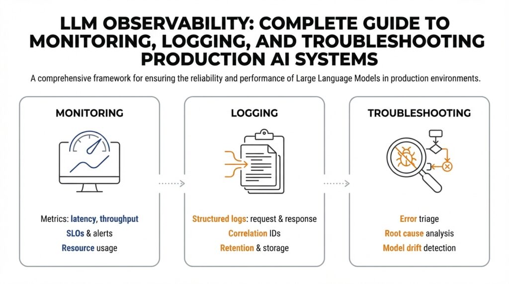
What is LLM observability
Imagine you just pushed an LLM-powered feature to users and, overnight, some responses start making no sense. You need LLM observability—our toolkit for watching, understanding, and fixing large language model behavior in real time. Observability means we can infer what’s happening inside a system from the outside: by collecting signals like metrics, logs, and traces we can spot performance drops, hallucinations, or prompt drift. In the world of production AI systems, observability pairs monitoring, logging, and troubleshooting so you aren’t flying blind when the model behaves unexpectedly.
Think of observability as a richly labeled dashboard that tells a story about your model. Monitoring (continuous checking of numerical indicators like latency, error rates, or token usage) gives you high-level health signals; logging (detailed records of requests, prompts, responses, and metadata) gives you the verbatim evidence you can read; traces or request-level telemetry show the path of a single interaction through your stack. Define a metric as a quantifiable measure (for example, 95th-percentile latency); define a log as a time-stamped record of an event; define a trace as a connected sequence of events for a single request. Together these signals let us ask and answer the key questions: is the model slow, wrong, or biased?
Let’s make this human. Picture a car’s dashboard: the speedometer is like a latency metric, the check-engine light is an alert, and the dashcam footage is your logs. If the car starts stalling, monitoring tells you there’s a problem, logs show what happened just before the stall, and traces reveal whether the fuel pump or ignition failed. In an LLM, a “stall” might be a sudden rise in incoherent answers, a spike in unsafe content, or a pattern where certain inputs consistently trigger hallucinations. Logging the full prompt, response, model version, and user context gives you the clues needed to reconstruct the failure.
Observability for LLMs is different from traditional application observability because models are probabilistic and context-dependent. A single query doesn’t always have one correct outcome, so comparing outputs requires behavioral metrics—things like response quality scores, factuality checks, or policy-violation rates—rather than just pass/fail. Monitoring infrastructure metrics (CPU, GPU, memory) remains important, but it’s not sufficient: you need semantic signals about the model’s behavior and data signals about input distribution shifts. This is exactly why logging and automated behavioral testing are essential complements to metric-based monitoring.
What signals should we collect right away? Start small and useful: request metadata (timestamps, model version, prompt ID), input and output pairs, quality ratings (human or automated), latency percentiles, and policy/flag tags for safety incidents. Add synthetic probes—automated queries designed to test known failure modes—and canary deployments that compare new model versions against a stable baseline. When we say tracing here, we mean capturing the lifecycle of a request across components so you can see whether the issue originated in the prompt engineering, the model layer, or downstream parsing logic.
How do you troubleshoot when something goes wrong? First, reproduce the issue using logged inputs or synthetic tests so you can observe it deterministically. Then narrow your scope: compare logs and metrics across model versions, prompt templates, or user cohorts to isolate variables. Use A/B tests and rollback mechanisms to limit exposure while you investigate. Finally, iterate: add targeted logging or probes for the suspected failure mode, tune prompts or guardrails, and validate the fix with both automated checks and human review.
Now that we’ve mapped what observability looks like and why it matters, the next step is to build the specific monitoring dashboards, logging conventions, and alerting rules that fit your product and risk profile. With thoughtful LLM observability in place, you and your team will move from reacting to surprises toward understanding, anticipating, and preventing them—so your production AI systems behave reliably for the people who depend on them.
Metrics, logs, and traces
Building on this foundation, imagine you wake up to an alert that something in production feels off — latency creeping up, or answers suddenly losing factual grounding. In that moment we rely on three kinds of signals to tell the story of what happened: numerical measurements (numbers we watch over time), event records (the readable snapshots of requests and responses), and request-level traces (the timeline that follows one interaction through your system). LLM observability becomes real when those signals let you move from “there’s a problem” to “here’s why” without guessing.
First, let’s talk about the numerical measurements you’ll lean on. Think of a measurement like a dashboard gauge: latency percentiles (e.g., p95), error rates, token usage, and behavior-focused metrics such as factuality score or safety-violation rate. Define a Service Level Objective (SLO) — a target like “p95 latency under 500ms” — so you know what counts as acceptable. Labels or tags (small pieces of metadata like model version, prompt template, or user cohort) let you slice these numbers; but watch cardinality — too many distinct labels makes queries slow and expensive. Start with a few high-signal labels and add more only when you have a clear hypothesis to test.
Now imagine opening the tape of a single request: event records are the readable evidence you’ll inspect. A good event record contains the prompt (or a safe, redacted form of it), the model response, timestamps, model and deployment versions, and a unique request ID that ties records to traces. Structured logs (JSON-style fields) make automated queries and parsing much easier than freeform text. How do you decide what to log? Prioritize data that helps reproduce and reason about failures: inputs and outputs, decision flags, and any automated quality checks; redact or hash personally identifiable information (PII) at ingestion to protect users and comply with policy.
Tracing follows that single request as it flows through components — prompt preprocessing, the model call, post-processing, and downstream services. Instrument each stage with spans (timed segments of work) and propagate a trace ID so you can see where time is spent or where errors originate. Low-overhead sampling keeps costs manageable: capture full traces for errors and a fraction of successful requests, and use full-fidelity tracing for deploys or suspected regressions. The trace is where you’ll see whether a hallucination came from a prompt rewrite, a token-truncation step, or a post-processing bug.
The real power comes when you correlate these signals into a debugging story. An anomaly alert on a measurement points you to the right time window; logs give you concrete inputs and responses to inspect; a trace tells you which microservice or stage introduced the change. For example, a sudden rise in incorrect factual responses might trace back to an automated prompt template change — logs show the template, traces show the new preprocessing path, and measurements show the cohort that was most affected. Make this workflow cheap and fast by assigning unique prompt IDs, version tags, and automated markers for synthetic probes so you can compare canary traffic against baseline.
Cost, retention, and privacy will shape how you implement all of this. Raw request storage is expensive: keep aggregated behavioral metrics long-term, retain full raw logs for a rolling short window, and store sampled raw records for longer-term trend analysis. Apply redaction rules at ingestion and encrypt logs at rest. Consider an incident-first strategy: increase sampling around anomalies automatically, then export the full context for post-mortem analysis.
With these practices in place, you’ll turn vague alerts into actionable stories quickly. Start by instrumenting a small set of behavioral measurements, adopt a structured logging schema with request IDs and redaction, and add tracing around the model call and preprocessing steps. That combination — timely measurements, readable records, and end-to-end traces — is the working toolkit that lets us detect, reproduce, and fix LLM issues with confidence as we build safer, more reliable systems.
Instrumenting LLM calls
Imagine you just deployed a feature and you want to know, for every user interaction, not only that the system responded but why it answered the way it did. Building on our discussion of LLM observability, instrumenting means adding the small sensors and labels around each model call so we can later ask useful questions: which prompt produced which output, which version of the model was used, and how long each step took. Think of instrumenting like stitching a numbered tag onto every parcel that passes through a sorting facility: later you can trace where it slowed, who touched it, and what changed in transit. This upfront tagging pays for itself the moment responses start changing in tone, accuracy, or latency.
The first practical decision is: what to capture at the model call boundary. Include a stable request ID that follows the interaction through preprocessing, the model call, and post-processing so you can tie logs and traces together. Record the model and deployment version, prompt template ID (not full PII), full or redacted input and output as policy allows, token counts (input, output, total), and all decoding parameters used (temperature, top-k, top-p). Also capture timing (client send, model receive, model send, server receive), status (success, timeout, error), and cost or token usage metadata so you can correlate behavior with expense.
Next comes how to add these signals without slowing the system: wrap the model client in a lightweight middleware layer. A middleware (a small piece of code that intercepts requests) attaches the request ID, starts a timer, and injects any tracing headers before calling the model API; when the response returns it records latency and any returned model metadata. This wrapper is the place to enforce redaction rules (hash or remove PII), to sample large payloads selectively, and to enrich records with contextual labels like user cohort or feature flag. Treat this wrapper like a recipe step: keep it small, test it in canary traffic, and iterate when you see gaps in observability.
Structured logging matters more than verbose logs. Use a consistent JSON schema for model-call records so automated systems can parse and query them later: a short description of a good schema would include request_id (string), timestamp (ISO 8601), model_version (string), template_id (string), input_tokens (int), output_tokens (int), duration_ms (int), response_text (string or hashed), safety_flags (array), and sample_rate (float). Declare the schema once in your team and validate writes; that makes it trivial to build dashboards that slice by template, model version, or user cohort without chasing inconsistent field names. Structured logs turn scattered evidence into searchable stories you can act on.
Tracing is the map that shows where time and errors are spent. Create a span specifically around the model call so you can separate network or API-side latency from your own preprocessing and post-processing work; propagate a trace ID through async queues and downstream services so the full lifecycle of a request is visible. Use adaptive sampling: capture full payloads and high-fidelity traces for errors and anomalies, and keep lightweight summaries for routine traffic. This approach keeps costs manageable while giving you the fidelity you need during incidents.
What signals tell you the model is misbehaving, and how do you choose them? Combine behavioral signals—automated factuality checks, safety classifiers, semantic similarity to expected answers, and human ratings—with operational metrics like p95 latency and token usage. Run synthetic probes and canary experiments that exercise known failure modes and tag those requests so you can compare canary metrics against baseline traffic. When you see divergence in any of these signals, the instrumentation we described lets you jump straight from an alert to the exact prompt, parameters, and trace that caused it.
Finally, plan for cost, privacy, and actionability so instrumenting serves operations, not noise. Define retention policies (shorter for raw text, longer for aggregated metrics), align logs with SLOs so alerts are meaningful, and automate increased sampling when an SLO breach or anomalous signal occurs. With these controls in place, instrumenting the model call becomes the connective tissue between monitoring dashboards and post-mortems, and it sets up the next step: building dashboards, alerts, and automated mitigations that let us move from noticing problems to resolving them quickly.
Monitoring quality and drift
Imagine you roll out an LLM feature and, after a week, answers start to feel off — shorter, less factual, or oddly repetitive. Right away you care about monitoring quality and spotting model drift so users don’t lose trust. Building on our LLM observability foundation, this is the place where semantic checks meet time-series alerts: we’ll walk through what to watch, how to detect shifts, and what to do when behavior changes.
First, let’s meet the characters in this story: data drift, concept drift, and prompt drift. Data drift (a shift in input distribution) happens when the kinds of queries you receive change — like sudden jargon from a new user cohort. Concept drift (a change in the relationship between inputs and correct outputs) occurs when the world moves underneath your model — for example, new facts, policies, or product features that make previous answers wrong. Prompt drift (changes to templates or user context) is when variations in phrasing cause consistent behavioral shifts. Defining these terms up front helps us pick the right detection tools.
Now ask the practical question: how do you detect drift before it becomes a user-visible problem? Start by instrumenting quality metrics beyond latency and errors: human or automated quality scores, factuality checks, safety-flag rates, and semantic-similarity measures against a ground-truth set. A quality metric is simply a numerical score that reflects how useful or correct outputs are (for example, a 0–1 factuality score). Track these metrics in rolling windows (1h, 24h, 7d) and compare them to baseline performance so you see gradual declines as well as sudden spikes.
One concrete detection technique uses embeddings as a thermometer for input distribution. Compute vector embeddings (numeric representations of text) for a baseline dataset and for recent traffic, then measure cosine similarity or centroid distance between the two distributions. If the average similarity drops past a chosen threshold for several windows, that’s a signal of data drift. This method is friendly to beginners: think of embeddings like fingerprints for text — when fingerprints stop matching the baseline, something has changed.
Statistical tests and behavioral checks give extra confidence. Simple tests like population-shift checks (e.g., Kolmogorov–Smirnov-style comparisons) detect distribution changes in numerical features such as token counts or intent scores. Complement those with behavioral probes: run synthetic queries that exercise known failure modes and compare model outputs against expected answers. Canary experiments that route a small percentage of traffic to the new model let you compare drift signals side-by-side with a stable baseline without exposing everyone.
When should an anomaly become an alert? Avoid flapping by requiring persistence: trigger alerts only when quality metrics breach thresholds over multiple consecutive windows or when multiple signals (e.g., embedding drift plus rising safety flags) co-occur. Define SLOs for behavioral metrics — for example, “average factuality > 0.85 over 24 hours” — and create tiered responses: a low-priority ticket for transient blips and an immediate incident for sustained breaches that impact critical cohorts.
Once you detect drift, follow a short investigation playbook so you don’t chase ghosts. Reproduce the issue with logged inputs and synthetic probes, slice by model version and prompt template to isolate cause, and inspect traces to see if pre/post-processing changed. Mitigate quickly with options like rolling back to a previous model, toggling a prompt template via feature flags, or routing suspect traffic to a human-in-the-loop flow while you diagnose.
Finally, make drift monitoring a continuous practice, not an occasional audit. Maintain a small labeled validation set that reflects high-value queries, budget regular labeling to refresh that set, and automate retrain or fine-tune triggers only after human review. Sampling strategies and privacy-preserving redaction keep costs and legal risk manageable while preserving the signals you need.
With these pieces in place — targeted quality metrics, embedding-based drift checks, canaries, and a clear remediation plan — you turn vague degradation into reproducible incidents we can fix. Building on our instrumentation work, the next step is mapping these signals into dashboards and automated alerts so the team can act quickly when drift first whispers and before it shouts.
Cost, usage, and latency
Building on this foundation, think of LLM observability, cost, usage, and latency as the three knobs you must tune when moving from a prototype to a product. You’ve already instrumented calls and captured traces, so now we learn how those signals translate into dollars and user experience. Picture a crowded kitchen: simmering pots are like background batch jobs that consume compute cost, the chef’s reaction time is your latency, and the number of dishes requested is your usage — all three affect whether diners leave satisfied. How do you balance cost, usage, and latency in practice?
First, let’s name the players so we can reason about trade-offs clearly. Cost is the money you spend on model inference, storage, and observability tooling; usage is the volume of requests and token usage (the number of input and output tokens consumed); latency is the time from a user’s request to the first useful response. Defining these terms helps you ask practical questions: which users care about latency most, where are tokens being wasted, and which logs are essential to retain? With those answers we can choose targeted optimizations instead of broad cuts that harm quality.
Cost is driven by model choice, token usage, and data retention. Larger models cost more per token, long retention of raw requests increases storage bills, and high-fidelity tracing multiplies billing at scale. Treat cost like a household budget: keep recurring essentials, defer long-tail spending, and pay for higher fidelity only when you need to investigate incidents. In practice that means keeping aggregated behavioral metrics for months, raw request storage for a short rolling window, and sampled payloads for trends; instrument token usage at the model boundary so you can attribute expense back to features and prompt templates.
Usage patterns offer the levers to reduce cost without hurting users. Route low-risk, high-volume queries to smaller, cheaper models and reserve the largest models for critical or complex tasks. Optimize prompts to trim unnecessary context and reduce token usage; think of prompt design like editing a message: fewer, clearer words cost less and often yield better answers. Add caching for repeated queries, batch similar requests when latency allows, and use adaptive sampling — record full payloads for errors and a fraction of successes — to keep observability useful but affordable.
Latency is often the most visible user pain point, and it’s also where observability shines. Use the traces you already capture to separate network, preprocessing, model inference, and post-processing time so you know where to act. If p95 latency is your SLO, a small increase in model size may push that number over the threshold even if median latency looks fine; we care about tails because they drive user frustration. Mitigations include streaming partial responses to the client, moving nonblocking work to background jobs, parallelizing safe preprocessing, and selectively using asynchronous UX patterns when exact answers can arrive later.
Finally, tie these ideas into operational guardrails so trade-offs are repeatable. Build cost-aware alerts and quotas that trigger when token usage or spend rate exceeds budgeted levels, and create routing rules that automatically fall back to cheaper models under sustained load. Use canaries and synthetic probes to measure cost and latency impact before full rollout, and increase sampling only during incidents so you get the evidence you need without permanent bill shock. With cost allocation, usage telemetry, and latency SLOs working together, you can make informed decisions that protect both user experience and your budget while keeping the observability data you need to improve over time.
Alerting and incident runbooks
Building on this foundation of LLM observability, imagine you wake to a notification and your stomach drops because the model has started answering with drifted facts or unsafe phrasing. An alert, in plain terms a notification triggered when a monitored metric crosses a threshold or an anomalous pattern is detected, is your early-warning bell; an incident playbook (also called a runbook, a step-by-step guide for responding to an operational problem) is the map you follow when that bell rings. How do you know which alerts are real and which are noise? That question will shape every rule you write and every page in the playbook we keep closest at hand.
Your first job is to make alerts meaningful instead of noisy. Treat alerting like setting a smoke alarm that doesn’t go off when you burn toast: prioritize signals tied to Service Level Objectives (SLOs) — the measurable targets we use to define acceptable system behavior — and combine complementary signals so a single blip doesn’t cause panic. Instead of firing on one metric alone, require two or three correlated indicators (for example, a drop in automated factuality score plus increased safety flags and a p95 latency breach) before an on-call rotation is paged. That approach reduces false positives while keeping monitoring sensitive to real regressions.
Designing the content of the runbook is next: write clear, short triage steps that anyone on the team can follow under pressure. Start with an immediate checklist that states what to capture first (time window, sample request IDs, model version, prompt template ID, and recent deploys), then provide diagnostic commands or dashboard links, and finally list quick mitigations such as toggling a feature flag or routing traffic to a baseline model. Define roles up front — who is the incident lead, who owns customer comms, who runs rollback — and include communication templates and escalation timing so nobody is guessing at 02:00.
Make the playbook operational by baking in automation and testing it with game days. Automate low-risk mitigations where safe: for example, an alert that satisfies a pattern can automatically increase sampling for raw requests, enable additional logging, or route suspect queries to a smaller model or human review queue. Treat the runbook as living code: keep it versioned alongside deployments, add unit-like smoke tests for the playbook’s critical steps, and rehearse scenarios regularly so the team’s muscle memory is tuned and the steps that look good on paper actually work in production.
Because LLMs are context-sensitive, attach rich context to every alert so triage is fast and evidence-rich. Include one or more sample request IDs with redacted input/output, the model and deployment tags, prompt template identifiers, a recent trendline for the relevant behavioral metric (factuality, safety-violation rate, semantic-similarity drift), and any synthetic probe results that exercise the suspected failure. Remember privacy: redact or hash PII at ingestion so alerts remain actionable without exposing sensitive data. These attached artifacts turn an abstract alarm into a reproducible debugging story.
Finally, build feedback loops so incidents improve observability instead of repeating the same confusion. After every event run a concise post-mortem that captures root cause, the timeline of alerts and runbook actions, and changes you’ll make to thresholds, telemetry, or the playbook itself. Feed those lessons back into monitoring: add new synthetic probes, adjust SLOs, and automate mitigations where recurrence risk is high. With this cycle you make alerting smarter and runbooks shorter, which means future incidents are faster to contain and easier to resolve.
With these practices — signal-aware alert rules, concise playbooks, safe automation, and incident-driven observability improvements — you turn noisy notifications into predictable operational work. In the next section we’ll map these signals into dashboards and automated mitigations so the team can see what matters and act before a small drift becomes a user-visible outage.