What Is DQN?
Imagine you are trying to teach an agent to play a game using nothing but the screen in front of it and a score that rises or falls over time. That is the problem a Deep Q Network, or DQN, was designed to tackle. In plain language, DQN combines Q-learning—a reinforcement learning method that learns how good each action is in a given situation—with a deep neural network, which is a layered model that can learn patterns directly from data. The original DeepMind paper described it as a model that learns control policies directly from high-dimensional sensory input, using raw pixels as input and predicted future rewards as output.
Building on that idea, the big breakthrough is not that DQN learns by trial and error, but that it learns from messy visual experience without needing hand-built features. Before this approach, reinforcement learning often depended on carefully designed inputs, which made it harder to scale to complicated environments. DQN changed the story by letting the network discover useful representations on its own, then using those representations to choose actions. In the Nature paper, the same basic agent was trained on classic Atari games and learned directly from pixels and game score, which showed that the method could handle a far more realistic stream of sensory data than older RL methods.
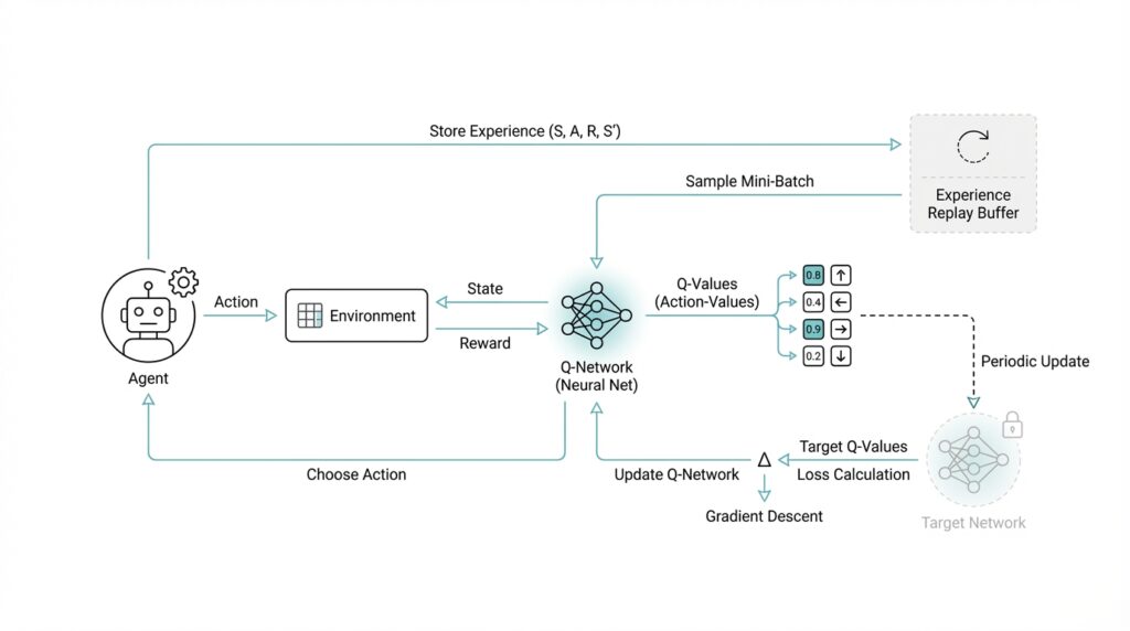
Here is where things get interesting: DQN does not learn well if you feed it one game frame after another in order, because consecutive moments in a game are highly correlated, like reading every word of a sentence without ever pausing to think. To reduce that problem, the original algorithm uses experience replay, which is a memory buffer that stores past transitions and samples them at random during training. That random sampling breaks up the correlation in the data and makes learning steadier. The paper also keeps the target value based on the previous network weights fixed while computing each update, which stabilizes training in the same way an answer key helps you compare your work before you move on to the next problem.
So how do you use DQN to make a decision in practice? The network outputs a Q-value for each possible action, and a Q-value is simply a score that estimates how much future reward you can expect if you take that action now. The agent then picks the action with the best value most of the time, while still exploring occasionally so it does not get stuck repeating the same behavior forever. This is why DQN fits naturally in environments with a finite set of choices, like Atari controls, where the action set is discrete rather than continuous. Think of it like a child learning a board game: first they try moves, then they remember which moves usually lead to better outcomes, and eventually they start choosing the stronger move more often.
The reason DQN matters is that it turns reinforcement learning into a bridge between perception and decision-making. In the Nature paper, the deep Q-network learned policies from high-dimensional sensory input and reported performance comparable to a professional human games tester across 49 Atari 2600 games. That result made DQN a landmark because it showed that a single model could learn across many tasks without handcrafted game-specific features or a separate rulebook for each environment. In other words, DQN is not just a neural network and not just Q-learning; it is the combination of both ideas, plus a few stability tricks, that makes the whole system work.
If you want the simplest mental picture, keep this one: DQN is a learner that watches what is happening, assigns a value to each possible move, stores old experiences to study later, and updates itself carefully so the learning does not wobble. Once that picture feels familiar, we can move from the idea of DQN itself to the mechanics of how its training loop actually works.
Set Up the Environment
Building on this foundation, the next thing we need is a clean place to run a DQN experiment without the rest of your machine getting tangled up in it. The easiest way to think about a Python virtual environment is like a separate workbench: it keeps the packages for this project away from the packages in your other projects, which makes experiments easier to repeat and easier to fix when something breaks. In practice, you create that isolated space with Python’s venv module, then activate it before installing anything else. That one habit pays off quickly when you start moving between different reinforcement learning projects or different versions of the same library.
Once the workbench is ready, we can bring in the two main tools for a DQN environment setup: PyTorch and Gymnasium. PyTorch is the deep learning framework that will hold the neural network, while Gymnasium is the library that provides the reinforcement learning environments the agent learns from. PyTorch’s official install page lets you choose a CPU-only build or a CUDA-enabled build, which is helpful because a CUDA build can use an NVIDIA GPU for faster training when your hardware supports it. If you are asking, “How do I set this up so it works on my computer?”, the safest path is to follow the official install selector and pick the option that matches your operating system, package manager, and hardware.
From there, the environment itself becomes the stage where the agent practices. Gymnasium environments are created through gymnasium.make(), which loads a registered environment and wraps it with the right helper layers when needed. That is a useful detail because DQN does not learn in the abstract; it learns by interacting with a concrete environment step by step, observing states, choosing actions, and receiving rewards. If you are starting with a classic control task or a toy benchmark, Gymnasium makes that part feel like opening a saved game rather than building a simulator from scratch.
If you plan to follow the classic Atari path that made DQN famous, there is one extra piece to handle: the game ROMs, or read-only memory files, that contain the actual Atari game software. Gymnasium’s Atari documentation notes that the ROMs are not bundled automatically and that pip install gymnasium[accept-rom-license] installs AutoROM and downloads them for you. That sounds like a small detail, but it is the kind that can stop a first run cold if you miss it. So while the code may look ready, the environment is only truly ready when the emulator, the ROMs, and the Python packages all agree with one another.
Before you write the first training loop, it helps to do a quick health check. A good setup tells you three things: Python can import torch, Gymnasium can create the environment you want, and your hardware path matches your plan, whether that is CPU training for a small test or GPU training for faster iteration. That is the quiet part of a DQN project that saves you hours later, because most early bugs come from missing dependencies, the wrong environment ID, or a mismatch between your installed packages and the machine you are running on. Once those pieces click into place, the agent can begin learning in a stable sandbox, and we can turn our attention to the code that actually starts the training process.
Build the Q-Network
Building on this foundation, the Q-network is where the DQN idea turns into something you can actually hold in code. The job of this model is straightforward in spirit, even if the details take a moment to settle: it takes the current game state, looks at what is happening, and returns a score for each possible action. In the original DQN, that scoring function is a deep convolutional neural network trained to approximate the action-value function, and in PyTorch you normally package that network by subclassing torch.nn.Module, the base class for neural network models.
Before we stack the layers, we need the right kind of input. The DQN paper does not feed the network a single raw frame and hope for the best; it converts Atari images to grayscale, resizes them to 84×84, and stacks the four most recent frames together so the network sees a short window of recent history. That is a little like showing someone a few snapshots from the same scene instead of one frozen picture, so the model can infer movement, direction, and timing rather than guessing from a static image alone.
Now the image can move through the network like a traveler through a series of rooms, each room extracting a different kind of signal. The original architecture uses three convolutional layers, which are layers that slide small filters across the image to detect useful patterns: first 32 filters of size 8×8 with stride 4, then 64 filters of size 4×4 with stride 2, then 64 filters of size 3×3 with stride 1. After that comes a fully connected layer with 512 rectifier units, and “rectifier” here means a ReLU, or rectified linear unit, which keeps positive values and suppresses negative ones. The final layer is linear and produces one output for each valid action, so the network ends by handing you a separate Q-value for every move the agent can make.
That design choice is the heart of why the Q-network works so well in DQN. Earlier approaches sometimes fed both the state and the action into the network, which meant you had to run a separate forward pass for each candidate action; the DQN architecture avoids that by making the action scores the outputs instead of extra inputs. In practice, that means the model can evaluate all actions in one pass, which is faster and cleaner when the action set is small and discrete, like the buttons in an Atari game. If you have ever wondered, “How do you build a DQN model that can see a game screen and turn it into action scores?”, this is the answer: one state in, one Q-value per action out.
In code, that usually means you define the layers in __init__() and then describe the data flow in forward(). The layers become named parts of the model, such as convolution blocks and a final output layer, and PyTorch registers them automatically because they are attached to the nn.Module subclass as attributes. That structure matters because it keeps the model organized, lets PyTorch track parameters, and makes it easy to move the whole network onto a CPU or GPU without rewriting the logic by hand.
What you end up with is a model that feels simple once the pieces click: the input gives it a short visual memory, the convolutional layers turn pixels into features, the dense layer blends those features into a decision-making representation, and the output layer assigns a value to each action. DQN relies on this Q-network to do the heavy lifting, because every training update is really teaching the network to make better estimates next time. Once this structure is in place, we are ready to connect it to the training loop and watch those estimates improve step by step.
Epsilon-Greedy Exploration
Now that the Q-network can score each move, we still face the real question: how do you choose an action without becoming trapped by the network’s first guess? Epsilon-greedy exploration answers that by giving the agent two moods. With probability ε (the exploration rate), it picks a random action; with probability 1 − ε, it picks the action with the highest predicted Q-value, which is the score for expected future reward. In other words, epsilon-greedy keeps the agent curious without letting curiosity take over.
That balance matters because early DQN predictions are often rough, and a purely greedy policy can get stuck repeating a move that only looked good by accident. Think of it like learning a new city: if you always follow the first road that seems promising, you may never discover the shortcut around the block. The exploration versus exploitation trade-off is one of the central problems in reinforcement learning, and DQN inherits it directly from Q-learning. The original Atari DQN work showed that this kind of value-based learner could reach strong performance on many games, but it still depended on a careful action-selection strategy during training.
How do you use epsilon-greedy in practice? You let the agent make a small number of “mistakes” on purpose, because those mistakes are often the only way to uncover better long-term behavior. A random action may lead to a reward path the agent has never seen, and that new experience becomes useful training material later. This is especially important in DQN because the network is not memorizing a fixed script; it is learning from its own interaction history, one transition at a time. So epsilon-greedy is not noise for its own sake — it is controlled uncertainty that helps the learner collect a broader map of the environment.
There is also a rhythm to how epsilon-greedy exploration usually feels over time. Early on, when the agent knows very little, a higher ε gives it room to search and compare different outcomes; later, a lower ε lets the learned Q-values guide behavior more often. That gradual shift is a practical way to move from discovery toward confidence, and it matches the wider RL idea that you should explore while the policy is weak and exploit more as it improves. You can think of it like training wheels that slowly lift off as balance improves.
What causes DQN to stall? Very often, the exploration setting is part of the answer. If ε drops too quickly, the agent may stop looking around before it has learned enough, and if ε stays too high for too long, it keeps acting like a beginner even after the network starts to understand the task. The sweet spot depends on the environment, but the principle stays the same: use enough random actions to discover useful experience, then let the Q-network take the wheel more often. That is why epsilon-greedy exploration feels so small in code and so large in impact.
Once that pattern clicks, the training loop starts to feel much less mysterious. The network estimates value, epsilon adds a little purposeful unpredictability, and the agent’s experience becomes richer with every step. That is the bridge that lets DQN move from raw scores on a screen to smarter decisions over time.
Add Replay Buffer
Building on this foundation, the replay buffer is where DQN starts to feel less like a stream of one-step guesses and more like a careful student reviewing old notes. A replay buffer, also called experience replay, is a memory store that saves what the agent saw, what it did, what reward followed, and what the next state looked like. In reinforcement learning, that saved bundle is often called a transition or experience, and it gives the network a reusable record of the agent’s past. How do you make learning steadier when game moments arrive in order, one after another? You break that order on purpose and let the agent learn from a mixed stack of earlier moments instead.
That idea matters because consecutive frames in a game are highly similar, almost like reading the same sentence with only one word changed each time. If DQN learned only from the most recent step, the training data would be too correlated, meaning nearby examples would look so alike that the network could overreact to tiny changes. The replay buffer solves that by storing many experiences and sampling them at random later, so each training batch contains a blend of old and new situations. This random sampling helps the Deep Q Network see a broader picture of the environment, which makes the value estimates less noisy and the updates more stable.
Here is where the replay buffer becomes especially practical: it lets one experience teach the agent more than once. Instead of using a transition a single time and discarding it, DQN can revisit that memory many times in different training steps, which is much more efficient than starting from scratch every time. Think of it like a notebook of past attempts; each page still has value even after you move on to the next problem. The buffer also smooths out learning when rewards are sparse, because an important event from a few hundred steps ago can keep influencing training long after it happened. That makes experience replay one of the quiet but essential tricks behind the original DQN results.
In practice, the replay buffer has a fixed capacity, which means it can only hold so many transitions before it starts overwriting the oldest ones. That detail is important because it keeps the agent from being overwhelmed by stale experience while still preserving enough variety to learn from. At training time, we draw a mini-batch—a small random group of stored experiences—from the buffer and use it to update the Q-network. A mini-batch is just a manageable slice of data, and it gives the model enough variety to learn from without trying to process the entire memory at once. This is the same idea that makes the replay buffer useful in DQN: we want controlled randomness, not chaos.
There is also a subtle benefit that is easy to miss at first. Because the replay buffer keeps older experiences around, it gives the agent a chance to learn from rare events that might not show up often in the current stream of play. If a surprising state led to a big reward or a dangerous failure, that memory can be sampled again later and shape the agent’s behavior more strongly than a one-time encounter would. That is why replay buffer design often becomes a balancing act between freshness and diversity. A smaller buffer remembers the recent past more strongly, while a larger one keeps a wider history alive for longer, and both choices change how the DQN learns.
Once this piece is in place, the training loop starts to make much more sense. The agent acts, stores the transition in the replay buffer, samples a random batch of past experiences, and uses those samples to adjust the network in a calmer, more reliable way. That is the bridge between raw interaction and stable learning, and it is one of the main reasons DQN works so well compared with a learner that only chases the latest moment.
Use Target Networks
Building on the replay buffer, we now face the next problem DQN has to solve: the model is learning from old experiences, but the value it is trying to learn is changing at the same time. That creates a moving target, which is a bit like trying to hit a bullseye while someone keeps sliding the board around. A target network is the calm, second copy of the Q-network that DQN keeps frozen for a while so the training signal has something steady to compare against. In the original DQN setup, this trick worked alongside experience replay to make training much more stable, and it was part of what let the agent reach strong results on Atari.
What is the target network doing, exactly? It is acting like the answer key while the main network, often called the online network, is still doing the homework. The online network keeps learning and changing its weights, but the target network copies those weights only at intervals and then stays fixed for a short stretch. That delay matters because the learner is no longer chasing a target that shifts every time the weights move; instead, it learns against a reference that stays still long enough for the update to make sense. Recent descriptions of standard DQN summarize it the same way: the target network is a copy of the online network’s weights, held fixed for several iterations before being replaced with a hard update.
So how does this work inside the actual update? When the agent sees a transition, the online network predicts the value of the action it took, while the target network estimates the value of the next state. The learning target is built from the reward plus a discounted estimate of future value, usually written as the reward term plus gamma times the maximum predicted Q-value from the target network for the next state. In plain language, the agent asks, “How good was this move, and how promising does the future look after it?” The target network answers the second half of that question without being distracted by the latest weight update.
That separation may feel small, but it changes the rhythm of learning in a big way. Without a target network, the model can get caught in a feedback loop where its own newest predictions immediately rewrite the labels it is trying to fit, which makes training wobble or even drift apart. With the target network in place, the DQN update becomes more like measuring your progress against a snapshot from a moment ago rather than against a mirror that moves with you. This is one of the core stability tricks that helped the original Deep Q Network learn directly from pixels and game score across dozens of Atari games.
In practice, the copy interval becomes a tuning choice. If you refresh the target network too often, the target starts moving again and the benefit fades; if you refresh it too slowly, the learner can lag behind the current policy and improve more cautiously than necessary. That is why many DQN implementations use a fixed hard-update schedule, copying the online weights into the target network every so many steps rather than on every gradient update. The exact timing is not magical, but the principle is: keep one network learning, and let the other network stay still long enough to steady the conversation between prediction and correction.
Once this idea clicks, DQN starts to feel less mysterious. The replay buffer gives the agent a richer memory to learn from, and the target network gives that learning a stable reference point so the updates do not spiral. Together, they turn a noisy stream of game experience into something the Deep Q Network can learn from with far less chaos, which is exactly why these two pieces sit at the heart of the algorithm.
Train and Evaluate
Building on the replay buffer and target network, this is the moment when DQN starts to look alive instead of abstract. You are no longer staring at a model diagram; you are watching a loop: observe the state, choose an action, receive a reward, store the transition, and learn from a sampled memory of past experience. The original DQN showed that this kind of end-to-end training can work directly from pixels and game score, and it proved the idea on 49 Atari games with one shared algorithm, one shared network design, and one shared set of hyperparameters.
How do you train a DQN without letting the learning wobble? First, the agent uses an epsilon-greedy policy, which means it takes a random action some of the time and the current best-scoring action the rest of the time. Then it stores each transition in replay memory, samples a random mini-batch from that memory, and computes a Bellman target, which is the training label built from the immediate reward plus an estimate of future value. The online network is updated with gradient descent, the step-by-step process that nudges the weights toward lower error, while the target network stays frozen long enough to keep the comparison stable.
That training signal is the quiet teacher in the room. It tells the agent whether a chosen move was better or worse than expected, even when the real payoff arrives several steps later. This delayed-credit problem is one of the reasons DQN needs replay and a target network in the first place: without them, the network would keep chasing its own moving predictions instead of learning from a steadier reference point. In the original paper, the learning process was tracked with curves for average score and predicted action-value, which is a helpful reminder that improvement often appears first as a smoother trend rather than a dramatic jump.
Once the learner has spent enough time practicing, evaluation becomes its own distinct scene. Here, we want to know what the policy can do when we stop leaning on randomness and let the learned values carry the decision-making as much as possible. In practice, that means running separate test episodes, keeping the environment settings fixed, and comparing the average performance across runs instead of trusting a single lucky game. That average-score view is common in Atari-style benchmarks, and DeepMind’s later writing on Atari evaluation makes the same point: one number is most useful when it summarizes performance across many games or many episodes.
What should you watch if the training curve rises but the evaluation curve refuses to follow? The usual clues are not mysterious bugs so much as mismatched learning conditions. If epsilon falls too quickly, the agent may stop exploring before it has seen enough variety; if the target updates are too frequent, the learning target can start moving again and destabilize the updates; if rewards are too sparse, the agent may need more diverse experience before the Q-values become meaningful. These are exactly the kinds of issues the replay buffer and target network were meant to soften, so when evaluation lags behind training, the answer is often found in those two stabilizers.
The practical rhythm is easy to remember once it clicks: train with purposeful noise, learn from shuffled memories, and evaluate with a calmer policy that shows you the agent’s real habits. That is what turns DQN from a clever idea into a usable reinforcement learning workflow. With that rhythm in place, we can next look at how to tune the learning setup when the agent needs to improve faster without becoming unstable.