Define Evaluation Scope
Building on this foundation, the first job is to define the evaluation scope before you compare any embedding models. If you skip this step, you end up asking one model to search clean PDFs, another to parse messy tables, and a third to answer narrow fact questions—and the comparison stops being fair. How do you know whether one embedding model is better for your RAG pipeline? You start by deciding what world the benchmark should represent. Benchmarks such as MTEB and BEIR were created because narrow, single-task checks miss broader retrieval behavior; MTEB spans 8 task types, 58 datasets, and 112 languages, while BEIR was designed as a heterogeneous zero-shot retrieval benchmark across 18 datasets and diverse domains.
The next boundary is the document collection itself, because real-world documents rarely look like tidy paragraphs in a notebook. In practice, you may be dealing with PDFs, tables, scan artifacts, multi-column layouts, or long reports that carry meaning across sections rather than inside one neat chunk. That is why benchmarks for real-world document analysis, such as UDA, evaluate on 2,965 documents and 29,590 expert-annotated question-and-answer pairs, and why newer retrieval suites keep stressing the importance of parsing as well as retrieval. The lesson is straightforward: if your production data looks like a messy filing cabinet, your benchmark should not behave like a polished textbook.
Once the document boundary is clear, we need to decide what kinds of questions the embedding models must handle. This is where the scope becomes more honest, because a system that does well on simple lookup questions can still stumble when the user asks something vague, paraphrased, or reasoning-heavy. BRIGHT was built for this exact problem: it focuses on real-world queries from diverse domains and shows that many of them require deeper reasoning than surface matching alone. So instead of testing only perfect keyword-style prompts, it helps to include short fact questions, multi-step questions, and awkwardly phrased questions that sound like something a real person would ask after skimming a report and still feeling unsure.
Now that we know what goes into the corpus and the query set, we need to define what success actually means. In a RAG system, the embedding model is usually doing retrieval work, not writing the final answer, so you should score retrieval quality first and generation quality second. That distinction matters because a fluent answer can hide a weak retrieval step, while a strong retrieval result gives the language model a better chance to stay grounded in the source material. UDA highlights that document parsing and retrieval are both important, and benchmark designs like REAL-MM-RAG explicitly call out realistic queries and accurate labeling as core properties of real-world retrieval. In other words, the scope should tell you whether you are judging search quality, answer quality, or both.
Finally, it helps to carve the benchmark into slices so you can see where each model shines or breaks. One slice might be document length, another might be OCR noise, and another might be whether the answer lives in a table, a figure caption, or a paragraph buried halfway down a report. This is where benchmarking top embedding models becomes genuinely useful, because the average score stops hiding the failure modes that matter in production. With that boundary drawn, you can compare embedding models for RAG on real-world documents with much more confidence, and the next step is to choose the metrics and test set that match the scope you just defined.
Prepare Document Corpus
Building on this foundation, the next step is to turn that broad scope into a working document corpus that feels like the real world instead of a polished demo. This is where benchmark design becomes tangible: you gather the files, preserve their quirks, and decide which parts of each document the embedding model for RAG will actually see. How do you prepare a document corpus for real-world documents without accidentally making it too clean, too small, or too easy? The answer is to treat the corpus like a museum archive, not a stack of shortcuts. You want the same PDFs, scans, tables, and long reports that your system will meet in production, along with enough structure to evaluate them fairly.
The first move is collection, because a corpus can only reflect reality if it comes from the right places. Instead of pulling only pristine text files, we include documents that mirror the messy mix users actually upload: contracts with dense clauses, research reports with figures, manuals with appendices, and scans where OCR had to do the heavy lifting. OCR, or optical character recognition, is the process that turns images of text into machine-readable text, and it matters because many real documents never arrive as clean copy. At this stage, the goal is not to beautify the data; it is to capture the document corpus in a form that still tells the truth about what the retrieval system must handle.
Once the files are in hand, we need to preserve their context before we start breaking them apart. That means keeping source metadata, page numbers, section titles, and table boundaries whenever possible, because those clues help you trace a retrieved passage back to its origin. Think of it like labeling boxes while moving house: if you strip away the labels, everything still exists, but nothing is easy to find later. This is especially important for benchmarking top embedding models, because a model should not get rewarded for finding a sentence while ignoring the structure that made the sentence meaningful in the first place.
Now comes the part that often feels trickier than it first appears: cleaning without overcleaning. We want to remove duplicate files, corrupted pages, and obvious extraction glitches, but we do not want to sand away the very features that make the benchmark realistic. A table, for example, may look awkward in raw text, yet that awkwardness is exactly what tests whether an embedding model can cope with layout-heavy content. So while we standardize formats and normalize obvious noise, we keep the document corpus faithful to its original shape, because a benchmark for real-world documents should reward resilience, not perfect formatting.
With the corpus stabilized, we can decide how to divide it for evaluation. This is where people sometimes get tempted to split documents too aggressively, but the benchmark works best when each file remains interpretable on its own terms. If a question depends on a figure caption, a footer note, or a paragraph on the next page, the corpus should preserve enough neighborhood information for the retrieval step to find it. In practice, that means setting clear rules for chunking, overlap, and document boundaries so the embedding models for RAG are judged on the same terrain they would face in production.
Finally, we make the corpus auditable. Every document should carry a stable identifier, a source record, and a version so future comparisons do not blur together different datasets or preprocessing choices. That sounds administrative, but it is what keeps the benchmark honest when you rerun it months later or compare models across revisions. Once the document corpus is assembled this way, you are no longer testing an abstract idea of search; you are testing retrieval against a grounded collection of real-world documents, which is exactly the kind of foundation the next stage needs.
Build Query Sets
Building on this foundation, we now turn the document corpus into questions that a real person might ask. This is where a benchmark starts to feel alive, because embedding models for RAG are not being tested on files alone; they are being tested on whether they can retrieve the right evidence when a user asks something specific, vague, or slightly messy. How do you build a query set that reflects real-world documents instead of a neat classroom exercise? You start by writing questions that sound natural, not artificially perfect, and by making sure those questions match the kinds of information people actually hunt for in reports, PDFs, tables, and scans.
The first step is to decide what each question is supposed to test. Some queries should be straightforward fact lookups, where the answer lives in one clear place and the challenge is finding it quickly. Others should require a little more effort, such as connecting two sections, interpreting a table, or following a paraphrased clue that does not repeat the document’s exact wording. This balance matters because a strong query set for real-world document retrieval should reveal both obvious wins and hidden weaknesses in the embedding model.
Now that we know the purpose of the questions, we can write them in the language of users, not annotators. That means varying length, tone, and phrasing so the benchmark includes short searches, conversational requests, and awkward phrasing that still makes sense to a human reader. Think of it like asking directions in a new city: sometimes you ask for the nearest train station, and sometimes you ask, “Where do I go if I need the office near the river with the blue sign?” A good query set captures that same range, because real-world documents are usually explored by people who do not know the exact terms the file uses.
We also want the query set to include hard cases, because easy questions can flatter a system that would struggle in production. A query might use a synonym instead of a keyword from the document, refer to a section indirectly, or ask about content that only appears in a caption, footer, or note. These cases are especially useful for benchmarking top embedding models, since embeddings are supposed to capture meaning, not just word overlap. When should you add these trickier questions? As soon as you want the benchmark to measure retrieval behavior that survives contact with real users, not just tidy prompts.
Once the questions exist, each one needs a trustworthy answer source. In a benchmark, that usually means identifying the exact passage, table cell, or page region that supports the answer so later scoring can check whether the retriever found the right evidence. This step is more like tagging treasure on a map than writing trivia cards: the question matters, but the hidden anchor is what makes the evaluation fair. If a query can be answered from multiple places, we need to decide whether we are testing broad retrieval, precise retrieval, or both, because embedding models for RAG behave differently depending on how tightly we define success.
It also helps to mix in negative space, which is a simple way of saying we should include questions that are not easy to solve by guessing. Some queries should point to information buried deep in the corpus, while others should require the system to ignore tempting but irrelevant passages. This keeps the benchmark honest, because retrieval systems often fail not by finding nothing, but by finding something plausible and stopping too soon. A thoughtful query set exposes those near-misses, and that is exactly what you want when comparing real-world document retrieval pipelines.
Finally, we should make the query set traceable and repeatable. Every question should carry an identifier, a source, and a reason for why it belongs in the benchmark, so future updates do not blur together different drafting choices. That discipline may feel invisible while you are creating the set, but it pays off the moment you rerun the benchmark on a new embedding model and need to know whether a score changed because the model improved or because the questions changed. With the queries anchored this way, the next step is to score how well each model retrieves the right evidence and see which failures matter most.
Benchmark Embedding Models
Now that the query set is in place, the real test begins: we ask how to benchmark embedding models in a way that rewards evidence retrieval, not lucky guessing. Imagine each model as a different reader walking into the same archive, searching the same documents, under the same rules. That means we keep the corpus fixed, keep the queries fixed, and keep the retrieval setup fixed so the comparison feels like a fair race instead of a moving target. When you benchmark embedding models for RAG, this is the moment where the benchmark stops being a spreadsheet and starts behaving like a mirror.
The next question is what we actually score, because not every metric tells the same story. Retrieval benchmarks commonly use Recall@k, Precision@k, Mean Reciprocal Rank (MRR), Mean Average Precision (MAP), and nDCG@k, where k is the cutoff for the top results we inspect. Recall@k tells you whether the right evidence appears somewhere in the shortlist, which matters a lot for RAG because the generator cannot use a passage it never sees. nDCG@k adds more nuance by caring about rank order, so a relevant document at the top counts more than one buried near the bottom.
With the scorecard chosen, we need to resist the temptation to trust the average alone. A model can look strong overall and still stumble on OCR noise, dense tables, long reports, or paraphrased questions that do not echo the document’s wording. That is why benchmark families like MTEB and BEIR were built to spread evaluation across diverse tasks and domains rather than reward one narrow retrieval pattern, and why BRIGHT and REAL-MM-RAG push further into reasoning-heavy and realistic query behavior. BRIGHT uses 1,384 real-world queries, while REAL-MM-RAG emphasizes multi-modal documents, realistic RAG-style queries, and accurate labeling.
This is where slice-level analysis becomes your best friend. Instead of asking only which embedding model wins overall, we ask where each model shines and where it breaks: short passages versus long ones, clean text versus OCR text, paragraph answers versus table answers, same-word matches versus paraphrased matches. That kind of breakdown turns a benchmark into a diagnostic tool, which is far more useful for real-world documents than a single leaderboard position. It also keeps you from celebrating a model that is excellent on easy lookup questions but fragile the moment a user phrases the request in a more human way.
To make the benchmark feel honest, we also need controls that keep the comparison grounded. Every model should use the same chunking rules, the same top-k cutoff, the same indexing approach, and the same corpus version, because changing those pieces can move the score as much as changing the model itself. It helps to inspect a small sample of retrieved passages by hand, too, because automatic metrics can miss a case where the top result looks relevant on paper but does not actually support the answer. That human check is especially valuable when the benchmark includes realistic queries, since realistic retrieval is often messier than clean evaluation data suggests.
Once those pieces are in place, benchmarking top embedding models becomes much clearer: you are no longer asking which model sounds best in theory, but which one consistently brings the right evidence to the surface under the same real-world pressure. From there, the next step is to compare the results against latency, cost, and downstream answer quality, because a strong retriever only matters if it fits the system you are actually building.
Measure Retrieval Metrics
Building on this foundation, we now need to answer the question that turns a benchmark into evidence: did the retriever place the right source material where the language model could actually use it? This is where retrieval metrics matter, because they tell us whether an embedding model for RAG is surfacing useful passages or merely returning plausible-looking text. If you have ever searched a messy folder and found almost the right file in the wrong place, you already understand the problem we are measuring.
The first metric most people reach for is Recall@k, where k means the number of top results we inspect. Recall@k measures how often the correct evidence appears anywhere in that shortlist, which is important because a RAG system cannot answer from a passage it never retrieves. For real-world document retrieval, this is often the clearest starting point: if the model misses the answer completely, no later step can rescue it. So when we ask, “How do you measure retrieval quality in a way that reflects production use?” recall is usually the first number we want to see.
Precision@k tells a different part of the story. Instead of asking whether the right passage appeared somewhere in the top results, precision asks how many of those retrieved passages are actually relevant. That distinction matters because a model can achieve decent recall by casting a wide net, but still waste space in the context window with distracting documents. In practice, we care about both: recall shows whether the model found the evidence, and precision shows whether it found it without filling the shortlist with noise.
Once those basics feel familiar, ranking metrics add another layer of realism. Mean Reciprocal Rank, or MRR, gives more credit when the first relevant result appears near the top, which matches how humans and downstream generation systems behave. Normalized Discounted Cumulative Gain, or nDCG@k, goes a step further by rewarding highly relevant results more than partially relevant ones and by favoring better rank order. Think of it like handing someone a stack of folders: finding the right folder immediately is much better than finding it after digging through a pile, even if both outcomes technically succeed.
That ranking detail is especially important for embedding models in RAG, because the generator usually reads only the top few chunks. If the best evidence sits at rank eight, the model may never see it, even though the retrieval system technically “found” it. This is why retrieval metrics should not stop at a single pass/fail score; they should show how much effort the model spends getting the right answer close to the top. In a real document pipeline, a small ranking improvement can make the difference between a grounded answer and a confident mistake.
We also want to measure retrieval in slices, not only in averages. A model may perform well on short paragraphs but struggle with tables, OCR-heavy scans, or questions that use synonyms instead of the document’s exact wording. When that happens, the overall score can hide the failure, even though those are the exact cases that trip up users in practice. So a strong benchmark for retrieval metrics breaks results down by document type, query type, and evidence location, which helps us see whether a model is genuinely robust or only good in easy conditions.
Another useful habit is to check evidence coverage, which tells us whether the retrieved passages actually contain the answer-bearing span. This is a practical layer of evaluation for real-world document retrieval, because a passage can look relevant at a glance while missing the one line that matters. By pairing evidence coverage with Recall@k, precision, MRR, and nDCG@k, we get a fuller picture of how well the embedding model supports RAG from the ground up. That combination keeps us honest about what the retriever is doing and what it is leaving behind.
Finally, the best retrieval metrics are the ones you can trust over time. If the corpus, chunking rules, or label quality change, the numbers may move for reasons that have nothing to do with the embedding model itself, so consistency matters as much as the score. Once you can read these metrics with that kind of caution, the benchmark becomes a dependable guide instead of a noisy leaderboard, and the next step is to interpret those scores alongside the costs and tradeoffs that shape the system you will actually ship.
Compare Model Tradeoffs
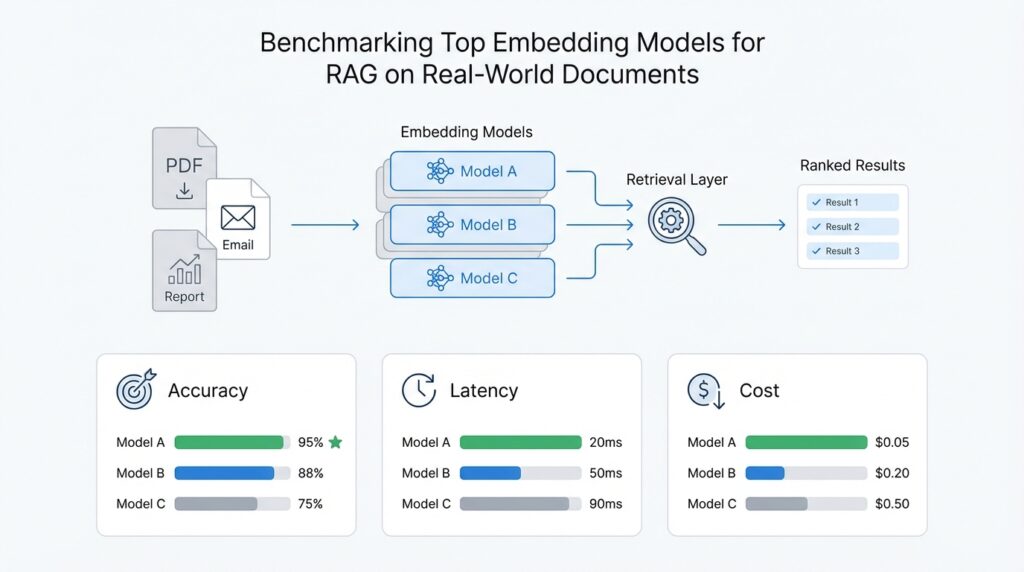
Building on this foundation, the next step is to compare model tradeoffs with the same calm eye you would use when choosing a tool for a home repair. The best embedding model for RAG is rarely the one that wins every metric; more often, it is the one that fits your documents, your latency budget, and your tolerance for complexity. How do you compare embedding models for real-world documents without getting lost in the numbers? You start by treating the benchmark as a map of tradeoffs, not a crown ceremony.
The first tradeoff is usually quality versus speed. A larger or more sophisticated embedding model may place more relevant passages near the top, especially on messy PDFs, paraphrased queries, and OCR-heavy text, but it can also cost more to run and take longer to index. That matters because retrieval is not happening in a vacuum; in a RAG system, every extra millisecond can slow the whole user experience, and every extra cent can scale into a serious bill. So when two models are close in Recall@k or nDCG@k, the faster model may be the better engineering choice even if it is not the absolute top scorer.
The second tradeoff is generality versus specialization. Some embedding models for RAG behave like versatile travelers: they work reasonably well across many kinds of text, languages, and question styles. Others feel more like specialists, excelling on one document type, such as technical prose or short fact lookup, while losing ground on tables, long reports, or heavily formatted scans. This is where the slice analysis from earlier becomes valuable, because a model that looks average overall may be the one that stays dependable across the widest set of real-world documents.
Then there is the question of semantic depth versus literal matching. A model with strong semantic understanding can recognize that “annual revenue” and “yearly sales” may refer to the same idea, which helps when users paraphrase their questions. But that same flexibility can sometimes pull in passages that feel related without being exact, especially when the document contains similar terms in several sections. In contrast, a model that leans more toward surface similarity may be less clever, yet more precise in narrowly structured corpora. This is why benchmarking top embedding models should not ask only “Which one is best?” but also “Which kind of mistake does each model make?”
Multilingual support adds another layer. If your corpus includes multiple languages, a model that handles cross-lingual search well may be worth a small drop in single-language score, because it keeps your retrieval system usable for more people. On the other hand, if your production data is almost entirely in one language, paying for broad multilingual ability may not buy you much. This is a classic real-world tradeoff in benchmarking: the strongest-looking model on paper is not always the most practical one for your actual document collection.
We also need to think about chunking behavior and context sensitivity. Some embedding models handle short, tight chunks very well, while others do better when the retrieved segment includes more surrounding context. That difference matters because real-world documents often hide the answer in a paragraph that only makes sense when you keep the heading, table caption, or nearby note intact. If a model performs well only after aggressive preprocessing, that may be a sign that the model needs more help than your pipeline can comfortably provide.
Cost and operational simplicity are tradeoffs too, even if they do not show up directly in a retrieval metric. A model that requires heavy preprocessing, special chunking rules, or frequent re-indexing can be harder to maintain than a slightly weaker model that fits neatly into your existing stack. In practice, the most useful choice is often the one that keeps the system stable under production pressure, not the one that looks best in a single benchmark run. That is especially true for benchmarking top embedding models on real-world documents, where the hidden cost of managing complexity can outweigh a small gain in score.
So the final comparison is not about declaring one universal winner. It is about matching the model’s strengths to the shape of your corpus, the kinds of questions your users ask, and the retrieval behavior your RAG system needs to survive day after day. When you read the benchmark this way, the numbers stop being a simple ranking and become a decision guide, which is exactly what you need before moving on to the practical implications for deployment and tuning.