Define Workload Requirements (learn.microsoft.com)
Before we pick a database, we need to slow the story down and look at how your application will live day to day. In database design, workload requirements are the clues that tell us what the system will do with data, how fast it must respond, and where it may struggle under pressure. How do you choose the right database if you do not know whether your app is mostly reading, writing, searching, or analyzing? Microsoft’s guidance starts with identifying access patterns first, because a single data store rarely handles every pattern efficiently.
The first layer is the shape of the data itself. We want to know whether the data is structured, semi-structured, or unstructured, because that tells us whether a rigid table-like model or a more flexible model makes sense. Then we look at the purpose of the workload: are we serving transactional data, which changes frequently and needs careful consistency, or analytical data, which is often queried in larger scans? At the same time, we ask about the access method, such as SQL, a REST API (a web-based interface for sending requests), or a software development kit, and about relationships like joins, graph traversal, or hierarchy. This is where schema flexibility, consistency, and data life cycle enter the picture: some workloads need strict rules, while others need room to evolve, age out, or move between hot and cold storage.
Now that we understand the data itself, we can talk about pressure. Nonfunctional requirements are the qualities the database must deliver while the app is running, and they often decide whether a design feels smooth or strained. Latency is how long a request takes to get a response, and throughput is how much work the system can complete over time; those two needs often pull in different directions. We also need to think about scale, meaning whether the workload grows upward on a bigger machine or outward across many machines, plus reliability, availability, failover, storage limits, and partitioning constraints. In plain language, this is the moment where we ask, “Will this database still feel responsive when real users, real traffic, and real growth arrive?”
A complete set of workload requirements also includes the practical realities around cost, operations, and control. Some teams want a managed service that handles patching, backups, and much of the upkeep; others need more direct ownership because of compatibility or administrative needs. You also want to think about security and governance early, not as an afterthought, because encryption, identity, auditing, network rules, and compliance boundaries can all shape which database options remain viable. And then there is team readiness: if your developers already know SQL, Python SDKs, or a specific driver ecosystem, that familiarity can reduce friction and lower risk. These are not side notes; they are part of the workload’s true shape.
This is exactly why two applications that share the same business goal can still need different databases. One app may need strict transactional consistency for orders or billing, while another may need flexible schema, fast search, or high-ingest telemetry. Microsoft’s guidance also notes that modern systems often use more than one storage model when access patterns or life cycles clearly diverge, because one database is not always the best fit for every job. So when you define workload requirements, you are not filling out paperwork; you are drawing the map that keeps the rest of the decision framework honest. Once that map is clear, we can move from “what does the workload need?” to “which database model matches those needs best?”
Map Access Patterns (learn.microsoft.com)
Building on that foundation, we now turn the map into something practical: the access patterns your application will actually use. Think of access patterns as the routes data takes in and out of your system—who asks for it, how often they ask, and what kind of answer they expect. Microsoft’s guidance starts here on purpose, because it recommends identifying patterns such as point reads, aggregations, full-text search, similarity search, time-window scans, and object delivery before you pick a storage model.
How do you map access patterns without getting lost in jargon? A helpful way is to imagine your database as a toolbox. You would not use a hammer for every job, and a single data store rarely fits every query shape efficiently, which is why Microsoft describes polyglot persistence as using multiple storage models when the workload calls for it. The key idea is not to spread data everywhere for its own sake; it is to match the tool to the question the application asks most often.
Now let us give those patterns a human face. A point read is a direct lookup for one record, while an aggregation asks for a total, average, or grouped summary across many records. Full-text search is the kind of query you use when words inside documents matter, similarity search helps you find things that are “close enough” in meaning, time-window scans focus on events from a specific slice of time, and object delivery is about serving files or binary content such as images, backups, or documents. Those shapes line up with different data store families: relational systems for consistent transactional work, search engines for text-heavy queries, vector-capable stores for similarity, time-series or analytics engines for timestamped data, and object storage for large files.
As we discussed earlier, the access method matters just as much as the data itself. Some workloads speak SQL, some use Gremlin for graph traversal, and others rely on a REST API (a web-based request interface) or an SDK (a software development kit, which is a packaged set of tools for coding against a service). Microsoft also notes that some platforms hide the engine behind a proprietary API layer, which can limit query flexibility and make integration harder, so the map should include not only what you query, but how you are allowed to reach it.
Taking this concept further, you also want to trace the shape of relationships, because joins, graph traversal, and hierarchical structures each pull the design in a different direction. If your app constantly follows links between entities, a relationship-centric model can save you from awkward workarounds; if your workload is mostly rigid transactions, a relational model tends to stay cleaner. The same logic applies to schema flexibility, consistency, concurrency, and life cycle: schema-on-write suits carefully controlled structures, while schema-on-read works better when the shape evolves over time, and hot data often deserves a different home than cold archival data.
In practice, the best way to map access patterns is to write down the dominant question each part of the system asks and the cost of answering it badly. A customer-facing order screen may need fast transactional reads and writes, a reporting job may need large analytical scans, and a search feature may need relevance ranking over text; those are different patterns, so they may deserve different storage models. Microsoft’s guidance says to combine models only where access patterns or life cycles clearly diverge, which keeps the design focused instead of fragmented. Once you can see those differences clearly, the next step is to turn them into a shortlist of Azure services that implement the right models.
Choose Data Model (learn.microsoft.com)
Building on that foundation, the next step in database design is to decide what shape your data should take before you ever choose a service. A data model is the storage pattern that tells your system how to organize, query, and update information, and Microsoft’s guidance emphasizes that a single store rarely handles every access pattern efficiently. That is why polyglot persistence means using more than one storage model only when the workload truly asks for different shapes or life cycles. Think of this as choosing the right container before we start packing the moving truck.
When your application needs strict consistency, the relational model is usually the first place we look. Relational databases store information in tables, define structure up front with schema-on-write (a fixed shape enforced before data is saved), and support ACID transactions, which means changes stay reliable even when many users update data at once. This model works well for orders, billing, inventory, and other multi-step business records where joins and constraints matter. The tradeoff is that large-scale growth often needs sharding or partitioning, and heavily normalized tables can make read-heavy views more expensive.
If your data arrives more like a living packet than a rigid form, the document model may fit better. A document store keeps related fields together, often in JSON (JavaScript Object Notation, a common text format for structured data), and lets each record evolve without forcing every row to look identical. That flexibility makes it a strong match for application objects, customer profiles, content catalogs, and APIs that change over time. In database design, this is often the “make the shape fit the story” option, especially when denormalized aggregates and multi-field indexing matter more than cross-table joins.
Other workloads care less about a full record and more about speed, density, or repetition. A key-value model stores one value behind one unique key, which is why it shines for caching, sessions, feature flags, and quick lookups where you want a fast answer and not a complicated query. By contrast, a column-family model groups sparse columns together so it can handle wide, write-heavy datasets efficiently, and a time-series model is tuned for timestamped metrics and windowed queries. How do you choose between them? A good mental picture is this: key-value is a labeled box, while column-family and time-series are shelves built for lots of small, repeated updates.
When relationships are the heart of the problem, the graph model becomes the clearer choice. Graph databases store data as nodes and edges, so they can follow connections through many steps without turning every question into a maze of joins. That makes them useful for social networks, dependency maps, and any workload where you keep asking, “What connects to what?” On the other end of the spectrum, analytics or OLAP (online analytical processing) models are built for massive historical scans and summaries, while object storage is better for large binaries, and search or vector models handle text relevance and similarity.
The practical test is to ask which need dominates: strict transactions, evolving JSON, fast lookups, sparse telemetry, deep relationships, or large-scale analysis. Once that dominant shape is clear, you can match it to the right data model first and then shortlist the Azure service that implements it. Microsoft also notes that some services support multiple models, but the safest choice is still the best-fit model, not the most feature-packed one. In other words, this step is where database design stops feeling vague and starts feeling like a set of clear trade-offs.
Set Consistency Needs (docs.aws.amazon.com)
Building on the work we already did around workload shape and access patterns, we now ask a narrower but very important question: how fresh does the data need to be when you read it? In database design, this is the heart of consistency needs, meaning the rule your system follows for whether a read must see the very latest write or can briefly lag behind. AWS’s guidance is clear that if your application can tolerate eventual consistency, a NoSQL approach may be a good fit; if it cannot, we need to look more carefully at stronger guarantees.
Think of eventual consistency like a shared notebook that takes a moment to circulate through the room. A writer finishes the note first, and everyone else catches up shortly after, which is fine when a small delay does not change the outcome. DynamoDB, for example, uses eventual consistency by default for reads, and those reads may not reflect a very recent write right away, but they will converge after a short time. That makes eventual consistency a practical choice for many distributed workloads where perfect immediacy is not required.
Strong consistency is the stricter version of that story. Here, you are saying, “If I just saved the data, I need the next read to show that saved value,” which is the safer choice for moments like checkout inventory, account balances, or a seat reservation screen. In DynamoDB, strongly consistent reads return the most up-to-date data from prior successful writes, but they are only supported on tables and local secondary indexes, not on global secondary indexes or streams. That limitation matters because it shows consistency is not only a business decision; it is also a database capability you have to verify.
Now we get to the tradeoff that often shapes database design decisions in the real world: stronger consistency usually costs more. AWS notes that eventually consistent reads use fewer resources than strongly consistent reads, and DynamoDB documents that eventually consistent reads cost half as much as strong reads for the same amount of data. In practical terms, that means you do not want to pay for strict freshness everywhere if only a few paths in the application truly need it. A good design often mixes both modes on the same table, using strong reads only where correctness depends on them.
When the application spans Regions, the story becomes even more interesting. DynamoDB global tables support multi-Region eventual consistency and multi-Region strong consistency, and AWS says the right choice depends on whether you value lower-latency writes with strong reads in a Region, or global strong consistency across Regions. In other words, once data starts living in more than one place, you must decide whether the “latest” version matters locally, globally, or both. That question can change the entire shape of the system.
So how do you use this in practice? Start by marking which parts of the application must never show stale data and which parts can afford a small delay without hurting the user. The first group usually includes transaction flows, state changes, and anything that would break trust if it looked outdated; the second group often includes feeds, analytics, dashboards, and background views where a brief lag is acceptable. Once you draw that line clearly, the rest of the database design conversation becomes much easier, because consistency stops being an abstract concept and turns into a concrete requirement you can match to the right storage model.
Compare Scale and Cost (learn.microsoft.com)
Building on this foundation, the next question is not whether your database can hold the data, but how it will behave when that data starts to grow. In database design, scale and cost are tied together like two sides of the same coin: every gain in capacity usually changes what you pay, how you operate, or both. You can think of it like choosing a vehicle for a long road trip. A compact car may be cheaper at first, but once the family, luggage, and miles add up, the real question becomes whether it still fits the journey.
So how do you compare scale and cost without getting lost in vendor details? First, look at whether your workload grows by getting bigger on one machine or by spreading across many machines. Scaling up means moving to a more powerful server, which is often easier to understand and manage, while scaling out means adding more nodes and sharing the load, which can handle growth better but usually adds design and operational complexity. That complexity matters in database design because a system that scales beautifully on paper can still become expensive if it needs careful partitioning, replication, or constant tuning to stay healthy.
Now that we understand the shape of scale, we can talk about cost in a more useful way than “which option is cheapest.” The sticker price of a database instance is only one part of the story. You also pay for storage, backups, network traffic, high availability, failover, and the staff time needed to keep everything running smoothly. A managed database service may cost more per hour than a basic self-managed server, but it can lower the total cost of ownership by removing patching, maintenance, and much of the day-to-day overhead. In other words, the cheaper box is not always the cheaper system.
This is where the real tradeoff starts to feel human. A small application may be perfectly happy on a modest setup, but the cost rises quickly if you have to overprovision resources “just in case” traffic spikes. Overprovisioning means buying more capacity than you need today so the system does not fall over tomorrow, and it is a common hidden expense in database design. On the other hand, an elastic platform that grows with demand can save money during quiet periods, but only if the scaling model matches your workload well enough that you are not paying for complicated architecture you barely use.
As we discussed earlier with workload requirements and access patterns, not every part of the application deserves the same treatment. A customer-facing transaction path may need low latency and steady performance, while reporting jobs, logs, or archives may tolerate slower access and cheaper storage. That is why scale and cost should be compared alongside the data model, not after it. When should you spend more for speed, and when should you save money by accepting slower access or colder storage? That question is often the difference between a design that feels balanced and one that feels like it is constantly fighting itself.
Taking this concept further, think about growth over time instead of only the launch day. The database design that works for 1,000 users may become wasteful at 100,000 if it relies on large fixed resources, and the design that is frugal today may become fragile when writes, reads, or stored data grow sharply. A good comparison of scale and cost asks what happens at each stage: early development, steady production use, and peak demand. Once you can see those stages clearly, you are ready to choose a database that fits not only the workload you have now, but also the one you are likely to inherit next.
Benchmark Candidate Databases (docs.aws.amazon.com)
Building on this foundation, we now put candidate databases through a real-world rehearsal. Imagine two options that both look promising on paper: the only reliable way to tell which one fits is to run the same workload against both and watch what happens. AWS recommends load testing to identify the metrics that matter for your workload and to confirm that the database can meet acceptable query times before you commit. That is the heart of benchmarking candidate databases: you are not guessing, you are measuring.
The first step is to establish a baseline, because you need something steady to compare against. AWS advises you to understand your current data characteristics and then experiment with different configurations instead of reaching immediately for a larger machine. In practice, that means looking at parameter groups, which are engine settings, along with storage options, memory, compute, read replicas, connection pooling, caching, and even eventual consistency. Think of it like tuning an instrument before a performance; the goal is to hear what each adjustment changes, not to hide every problem by turning the volume up.
Once the baseline is clear, test the traffic pattern itself, not only the database size. AWS recommends checking the current or expected peak transactions per second and then repeating the test at that level plus extra headroom, because weak spots often appear only under pressure. When possible, capture production-like traffic and replay it, since real user behavior is usually messier than a clean synthetic test. This is where database benchmarking becomes useful in a practical sense: the candidate that looks smooth in a demo may slow down, queue up, or behave unpredictably when requests arrive in bursts.
Read-heavy and write-heavy systems need different kinds of proof. For reads, the benchmark should show whether read replicas, caches, or dedicated accelerators actually reduce pressure on the primary database; for writes, it should reveal whether batching, queues, sharding, or larger instances are needed to keep throughput stable. AWS specifically warns against relying only on instance size, because a bigger server can conceal the real bottleneck instead of fixing it. If you are testing a service such as DynamoDB, hot partitions matter too, because one partition key can become the choke point when too much traffic lands in the same place.
You also want to benchmark how the system behaves as it scales, not just how fast it feels in a single snapshot. AWS recommends testing the impact of serverless or elastically scalable compute and considering connection management or pooling so the database is not overwhelmed by too many open connections. It also suggests looking at predictable traffic, sudden spikes, and quiet periods, because those patterns may call for scaling down during idle windows or using a service that grows and shrinks automatically. In other words, benchmarking candidate databases is really about finding the option whose performance stays understandable when the workload changes shape. With those measurements in hand, the shortlist becomes much easier to defend.