Understand Incremental Pipeline Stages
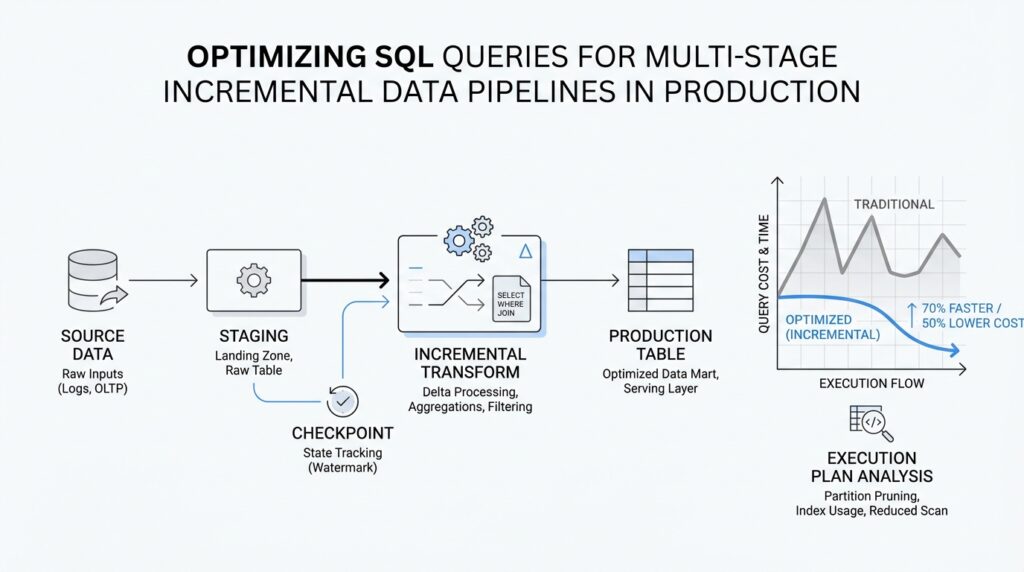
Now that we’ve set the bigger picture, it helps to look at the pipeline as a chain of small, moving rooms rather than one giant machine. In incremental data pipelines, each stage receives only the rows that changed, shapes them a little more, and hands them forward. That matters because SQL query optimization looks different when you are working in a production flow that runs over and over, not in a one-time report. If you have ever wondered, “Why is this query fast in testing but slow in production?” the answer often lives in the handoff between stages.
The first stage is usually the place where new data enters the system, and it sets the rhythm for everything that follows. Here, we are often reading from source tables, change logs, or event feeds, then filtering to the latest batch by a watermark, which is a marker that tells us how far we have already processed. Think of it like sorting through today’s mail instead of the whole post office archive. When this stage is lean, the rest of the pipeline starts with a small, clean set of rows, and that alone can cut the cost of every later join, filter, and aggregation.
Next comes the transformation stage, where raw data gets cleaned, standardized, and reshaped into something usable. This is where SQL can become expensive if we are careless, because small inefficiencies multiply across repeated runs. A common mistake is to apply the same filter or parse the same field again and again in multiple CTEs, or common table expressions, which are named query blocks that make SQL easier to read. In production, multi-stage incremental data pipelines work best when each stage does one clear job and passes along only the columns and rows the next stage truly needs.
After that, we often enter the enrichment stage, where the pipeline adds context from lookup tables or reference data. This is where joins can quietly become the most expensive part of the journey. We want to join on well-indexed keys, which are columns the database can search quickly, and we want to trim the data before the join whenever possible so we are not asking the database to match more rows than necessary. In practice, SQL query optimization here means asking a simple question: are we adding value, or are we dragging unnecessary data through the door?
Then comes aggregation, where many small records become summaries that are easier to store and analyze. This stage often feels like the payoff, because we turn noisy detail into counts, totals, averages, or daily snapshots. But aggregation over incremental data can be tricky, because we need to be careful not to recount old rows or miss late-arriving changes. The best production designs keep a clear boundary between fresh input and previously processed output, so each run updates only what changed instead of rebuilding everything from scratch.
Finally, the publishing stage writes the result to a table, a dashboard layer, or another downstream system. This is the moment where pipeline design and query behavior meet the real world, because a query that is elegant on paper can still cause trouble if it writes too much data too often. Partitioning, which means splitting a table into manageable chunks such as by date, can make these writes faster and cheaper because the database can update a smaller slice of data. In incremental data pipelines, the publishing stage is not just an ending; it is the handoff that decides whether the next run starts smoothly or inherits a mess.
What ties all of these stages together is the idea that each one should reduce work for the next. When we understand incremental pipeline stages, we stop treating SQL as one block of logic and start seeing it as a sequence of deliberate handshakes. That shift is what makes SQL query optimization practical in production, because we can tune each stage for its own job instead of hoping one giant query will do everything well. With that mental model in place, we are ready to look at how to measure where the time is really going.
Filter Early, Scan Less
When a production pipeline slows down, the trouble often starts before the real work even begins. In SQL query optimization for incremental data pipelines, we want the database to look at the smallest possible set of rows, because every extra row can ripple through joins, aggregations, and writes. How do we filter early and scan less? We start by placing the strongest filter where the engine can see it first, so the query plan can avoid scanning data that will never survive the next stage. PostgreSQL’s execution plans show different scan nodes, and partitioned systems like BigQuery can skip unused partitions when the filter matches the partitioning column.
That first filter matters even more when we are working with a watermark, the marker that tells us how far we have already processed. If we apply that watermark directly against the source table or change log, the database has a clear path to trim the search space before it touches the rest of the pipeline. The important habit is to write the filter so it stays visible, because a qualifying condition on a partition column can enable pruning, which means the engine scans only the partitions that might contain matching rows. In other words, the database can only skip work if we give it a filter it can recognize early.
The next place where work quietly piles up is in the columns we carry forward. A wide row is like a suitcase stuffed with things we never use again: it takes more effort to move, and it slows every downstream step. PostgreSQL notes that an ordinary index scan still has to fetch data from both the index and the heap, while an index-only scan can answer a query from the index alone without heap access, which is one reason tighter projections can matter. So when a stage only needs five fields, we should keep those five fields and leave the rest behind instead of dragging them through the whole chain.
Common table expressions, or CTEs, are another place where scan less can either happen or get blocked. In PostgreSQL, a non-recursive, side-effect-free WITH query can be folded into the parent query, which lets the planner optimize both levels together; if it is materialized instead, the database may have to build a temporary copy before it can apply the parent’s restrictions. That difference matters in incremental data pipelines, because a filter hidden behind a materialized step can force the engine to read far more rows than the final output needs. The safer pattern is to keep each stage narrow and readable, but not so boxed in that the planner loses sight of the row-reducing conditions.
Joins are where the benefit becomes easiest to feel. When we filter early, the join has fewer candidate rows to match, and that alone can turn a heavy step into a manageable one. PostgreSQL describes index scans as using scan keys derived from WHERE conditions, and its partition pruning support can remove partitions that cannot satisfy the query’s filter; in newer plans, even matching partitions can be joined more directly when the keys line up. So the practical question is not “Can this join work?” but “Can we make this join work on less data?” That is the heart of SQL query optimization in production.
Once we adopt that habit, every stage starts to ask the same quiet question: which rows can we rule out right here, before they cost us more downstream? That question is especially powerful in incremental data pipelines, because each run only needs the fresh change set, not the full history. The more we reduce the row count at the source, the less the database has to scan, join, group, and write later on. And when we are not sure whether the filter is actually helping, the next move is to inspect the plan and see whether the scan nodes really got smaller.
Partition Tables for Pruning
Now that we’ve learned to filter early, the next question is where those filters can do the most good. In SQL query optimization for incremental data pipelines, partitioned tables give those filters a place to land: PostgreSQL describes partitioning as splitting one large logical table into smaller physical pieces, while the partitioned table itself acts like a virtual shell with the real storage living in the partitions underneath.
That matters because pruning works like a bouncer at the door. If the WHERE clause matches the partition bounds, PostgreSQL can prove that certain partitions cannot contain matching rows and skip them entirely, which is why a query on a date range can avoid scanning older monthly partitions. The planner can do this during planning, and it can also prune again during execution when values are not known up front, such as parameters from a PREPARE statement or values coming from a nested loop join.
For incremental pipelines, this is where the design starts to feel practical instead of theoretical. If each run processes “today’s data” or “this batch’s data,” then partitioning by the same column that appears most often in your filters gives the optimizer a clean shortcut. PostgreSQL recommends choosing partition keys that commonly appear in WHERE clauses, because only clauses compatible with the partition bounds can prune unneeded partitions. In other words, the table should be shaped around the question you ask most often, not the one you ask once in a while.
There is a catch, though: more partitions are not automatically better. PostgreSQL warns that too many partitions can increase planning time and memory use, especially when a query still has to consider a large number of them after pruning. The sweet spot is a structure where pruning leaves only a small handful of active partitions, so the engine spends its effort on the rows that matter instead of carrying the overhead of the whole table layout. That balance is a quiet but important part of SQL query optimization in production.
How do you know whether pruning is actually happening? PostgreSQL’s EXPLAIN output is the flashlight here. You can compare plans with enable_partition_pruning turned on and off, and the docs show that a pruned plan may scan only the relevant partition instead of appending scans across many partitions. It is also worth remembering that pruning is driven by partition bounds, not by indexes alone, so you do not need an index on the partition key just to make pruning work; indexes help when you still expect to read a lot from a specific partition.
That distinction helps when you are thinking about production cleanup, too. PostgreSQL notes that an entire partition can be detached fairly quickly, which makes partitioning useful not only for pruning but also for removing old data in clean, low-drama chunks. For incremental data pipelines, that means the same structure that speeds up fresh reads can also make retention easier to manage, because old batches sit in their own containers instead of blending into one massive heap of rows.
Once the table is arranged this way, the rest of the pipeline has a better chance of staying small, focused, and predictable. Partition pruning does not replace good filtering, but it rewards it, and that is exactly the kind of feedback loop we want in production: smaller scans, narrower joins, and fewer surprises as new data keeps arriving.
Use Staging Tables Wisely
After we have filtered early and let partition pruning do its work, there is often one more place where the pipeline can either stay nimble or start to drag: the staging table. In SQL query optimization, a staging table is the waiting room between stages, a place where we can pause messy input, shape it, and hand it forward in a form that is easier to trust. That matters in incremental data pipelines because the goal is not to store everything forever in one giant intermediate layer; it is to create a small, useful checkpoint that helps the next step move faster.
The first reason to use staging tables wisely is control. When raw data arrives in awkward shapes, with nested fields, duplicate records, or half-finished updates, a staging table gives us a safe place to normalize that chaos before it reaches the rest of the flow. Think of it like unpacking groceries on the counter before putting them in the fridge: we can sort, clean, and group things where they are easy to see. In SQL query optimization, that extra pause can reduce repeated parsing, repeated casting, and repeated joins later on, which is often where production time quietly disappears.
A staging table also helps us separate one job from another. Earlier, we looked at each pipeline stage as a clear handshake, and staging tables support that idea beautifully when they stay narrow and purposeful. We want the table to hold only the rows and columns the next step actually needs, because every extra field adds storage, I/O, and mental overhead. What should a staging table contain in incremental data pipelines? Usually, the answer is: enough to make the next transformation reliable, but not so much that we are dragging the source table around in disguise.
That small design choice matters even more when a stage is reused. If a transformation is expensive, or if several downstream steps need the same cleaned dataset, a staging table can prevent us from recomputing the same logic over and over. Instead of asking the database to reread the source and redo the same filters, we pay the cost once and reuse the result. In practice, this can make SQL query optimization feel less like guesswork and more like setting down one sturdy stepping stone before crossing the stream.
Still, staging tables can become a trap if we treat them as a place to dump everything “for later.” A wide, overgrown staging layer can be just as costly as the source system we were trying to avoid. If the table is reused across batches, stale rows can blur the boundary between fresh and already-processed data, and that creates the kind of ambiguity that incremental data pipelines cannot afford. The safer habit is to make the lifespan of the table match its purpose: temporary when the work is short-lived, persistent only when we truly need a checkpoint for retries, auditing, or downstream reuse.
The way we write into the staging table also affects whether it helps or hurts. If each run inserts only the current batch, then the table stays small and predictable; if each run rewrites huge swaths of old data, we lose much of the benefit we gained earlier. For production SQL query optimization, the best staging design often looks boring in the best possible way: clear boundaries, predictable keys, and just enough structure for the next join or aggregation to work without surprises. That is especially important when the next step needs to match on a stable identifier, because a clean staging key keeps later logic from wandering through duplicates and partial updates.
When we use staging tables wisely, they become more than a storage trick. They give incremental data pipelines a place to slow down briefly, clean up the shape of the data, and then move forward with less friction. And once that intermediate layer is right-sized, we can start thinking about the next question in the journey: how do we merge, update, or deduplicate those staged rows without turning the whole pipeline into a bottleneck?
Tune Joins and Merges
When the pipeline reaches the handoff between staged rows and final tables, joins and merges decide whether the run feels light or sticky. In PostgreSQL, the planner picks a query plan for each statement, and EXPLAIN is how we see that choice instead of guessing. Why is this MERGE statement slow even though only a few rows changed? Often the answer is that the statement is asking the database to compare too many rows, or to compare them in the wrong shape. In SQL query optimization, this is the moment to make the merge path smaller before we try to make it clever.
The first thing we usually tune is the join type itself. PostgreSQL can use a nested loop join, a hash join, or a merge join, and each one tells a different story about the data. A nested loop walks one input row by row and probes the other side for each row, which can work well when the outer set is small and the inner side is easy to search. A hash join builds an in-memory hash table for one input and probes it with the other, while a merge join expects both inputs to arrive sorted on the join keys. In other words, the “best” join is the one that matches the shape of the rows we already have.
That is why filtering before the join still matters so much in incremental data pipelines. When we cut the outer side down early, the join has fewer rows to compare, and a nested loop has fewer passes to make over its inner input. When we keep the join keys narrow and the staged data trimmed, a hash join builds a smaller table and a merge join has less sorting work to do. This is the quiet payoff of SQL query optimization: every row we remove before the merge is a row the database never has to compare, sort, or move again.
Join order can also change the mood of the whole query. PostgreSQL can reorder many explicit joins on its own, but FULL JOIN constrains the order completely, and setting join_collapse_limit to 1 tells the planner to honor the written join order for explicit joins. That is useful when the default plan is wandering through a costly path, but it is also a sharp tool, so we should use it only when we have evidence that a specific order is better. If you have ever asked, “How do I make PostgreSQL join these tables in the order I want?” this is the lever the planner gives us.
MERGE deserves its own careful touch because it can INSERT, UPDATE, or DELETE in one statement. PostgreSQL also warns that only target-table columns that actually participate in matching should appear in the join_condition, because extra target-only conditions can change which action fires in surprising ways. If you combine both WHEN NOT MATCHED BY SOURCE and WHEN NOT MATCHED [BY TARGET], PostgreSQL performs a FULL join between the source and target, which means the join operators must support either a hash join or a merge join. That makes broad MERGE statements powerful, but also easier to overfeed with unnecessary work.
This is where the shape of the staging table starts to matter again. If the staging layer already holds only the current batch, the MERGE statement can compare a small source against a bounded target slice instead of walking the whole table like it is doing a census. If the join keys line up with indexes or natural sort order, PostgreSQL may be able to use an index scan or a merge join more efficiently; if not, it may need to sort the inputs first, and that cost shows up fast when the batch grows. The practical habit is to make the match columns stable, selective, and easy for the planner to reason about.
When we inspect the plan, we are looking for the little clues that tell us where the time is going. A materialize node can mean the planner is saving one side of a nested loop so it does not reread it over and over, and a merge join tells us the inputs had to arrive in order. If the plan shows a join stepping through far more rows than the batch should contain, that is usually the signal to tighten the filter, simplify the ON clause, or split the work so the merge only sees the rows that truly changed. That is the heart of SQL query optimization in this part of the pipeline: make the database compare less, not merely compare faster.
Inspect Plans and Metrics
At this point in the pipeline, the data is already trimmed and shaped, so the real question becomes: where is the time actually going? In SQL query optimization for incremental data pipelines, we do not want to guess from feelings or isolated test runs; we want to read the planner’s story and compare it with what happened in production. EXPLAIN shows the plan the PostgreSQL planner chooses, and that plan is a tree of nodes, with scans at the bottom and joins, sorts, or aggregations above them.
The first pass is EXPLAIN, but the more revealing step is EXPLAIN ANALYZE, which actually runs the query and reports real row counts and real execution time for each node. That is where we can spot the quiet mistakes: an estimate that is far from reality, a node that loops far more times than we expected, or a join that looks small on paper but grows expensive once the batch arrives. PostgreSQL also warns that EXPLAIN ANALYZE executes the statement for real, so data-changing queries should be wrapped in a transaction if you want to roll them back after inspection.
Once the shape of the plan makes sense, we turn to the smaller clues inside it. EXPLAIN (ANALYZE, BUFFERS) adds buffer-usage details, including shared blocks hit and read, local blocks, and temp blocks, which helps us tell the difference between a query that is CPU-heavy and one that is waiting on I/O. It also shows lines such as Rows Removed by Filter, which are especially useful in incremental pipelines because they reveal whether we are scanning too much data before the stage has a chance to narrow it down. If track_io_timing is enabled, PostgreSQL can also report time spent reading and writing blocks, which makes the I/O bottleneck much easier to see.
A single plan is useful, but recurring production work needs a broader memory. That is where pg_stat_statements helps: it tracks planning and execution statistics for statements across the server, grouping normalized queries together so we can see repeated offenders instead of one-off samples. Its view includes columns such as calls, total_plan_time, total_exec_time, rows, shared block hits and reads, temp block activity, and even WAL (write-ahead logging) metrics, which is exactly the kind of long-running evidence we want when a pipeline runs batch after batch. To use it, PostgreSQL requires the module to be loaded through shared_preload_libraries, and query identifier calculation must be enabled.
If we are asking, “How do I find the slow query in PostgreSQL without watching every run by hand?”, auto_explain is the answer worth knowing. It logs execution plans automatically for statements that cross a duration threshold, and it can include ANALYZE, buffer usage, WAL usage, and nested statements when configured to do so. That makes it a good production companion for SQL query optimization, because we can catch the plan as it actually appeared during a bad run instead of waiting to reproduce it later in a lab.
The practical habit is to compare these layers together, not one at a time. EXPLAIN ANALYZE tells us how one query behaved right now, BUFFERS and timing counters tell us whether the cost came from scanning, sorting, or writing, and pg_stat_statements tells us whether the same pattern keeps returning across many runs. In incremental data pipelines, that combination is especially powerful because the work changes from batch to batch, and we need to know whether a stage is healthy in general or merely lucky on one small sample. Once we can read both the plan and the metrics, we are ready to decide which part of the pipeline deserves the next fix.