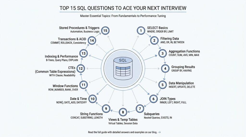
SQL Interview Basics
When you walk into an interview, the hardest part is often not writing SQL itself—it is recognizing what the interviewer is really testing. What are the SQL interview questions that trip people up the most? Usually, they are checking whether you can read a table of data, shape it into the result you want, and explain your choices clearly. The good news is that SQL interview prep becomes much less intimidating once you see the language as a small set of building blocks rather than a pile of memorized tricks.
The first building block is the SELECT query, which asks the database to return chosen columns from a table or from a joined result set. Think of SELECT as pointing to the rows you want, while WHERE acts like a gatekeeper that removes rows that do not meet a condition before the final result is returned. This is why beginners often feel surprised when a filtered query behaves differently from an unfiltered one: the database is not “changing” the data, only narrowing the view you asked for. ORDER BY comes last in that story, because it arranges the rows after the database has already found them.
Next comes the part that feels like matching puzzle pieces: JOIN. A JOIN combines rows from two tables when a shared value lines up, and an outer join can still keep unmatched rows by filling the missing side with NULL, which means “unknown” or “missing” in SQL. That detail matters in interviews because a tiny change in join type can completely change the answer, especially when the question asks you to include customers with no orders or employees without a department match. If you have ever wondered why a query returns fewer rows than expected, the join type is often the first place to look.
After that, interviewers often move into grouping, because grouping shows whether you understand how SQL summarizes data. GROUP BY collects rows that share the same value, and aggregate functions are calculations such as COUNT, SUM, or AVG that collapse many rows into one answer. WHERE filters individual rows before grouping, while HAVING filters the grouped results afterward, which is why HAVING is the right tool when you want “departments with more than five employees” instead of “employees with more than five something.” This is one of those SQL interview questions that looks small on the surface but quietly reveals whether you understand the order of operations.
NULL deserves its own attention because it behaves differently from ordinary values. In SQL, comparisons involving NULL do not produce a simple true or false result; they can produce a third outcome, often described as unknown, and that is why = NULL is not the same as checking for missing data. Once you know that, many interview mistakes start to make sense: a filter that looks correct can still exclude rows because the condition never becomes true. This is also why careful interview answers often mention IS NULL instead of treating NULL like an empty string or a zero.
Finally, you will often hear about indexes, and they are worth keeping in your pocket. An index is a database lookup structure that can speed up queries, especially when your filter or join condition matches the indexed column, though it also adds work when data changes. For interview purposes, the useful idea is not “indexes are magic,” but “indexes can help the database find fewer rows faster.” If you can explain that tradeoff in plain language, you are already speaking the language of strong SQL interview prep, and we can build from there into the trickier questions that mix joins, grouping, and filtering in one query.
Joins and Relationships
When you start working with SQL joins, it helps to picture two notebooks that are meant to tell one story. One notebook might hold customers, and another might hold orders, and the real question is how we connect the names in one place to the purchases in the other. That connection is the heart of table relationships in SQL, and interviewers love asking about it because it shows whether you can move between separate tables without losing the plot. If you have ever asked, “How do SQL joins work when the data lives in different tables?”, this is the moment where the pieces begin to click.
The first idea to hold onto is that a join matches rows through a shared value, usually a key such as a customer ID or product ID. A key is just a column that helps identify a record, and a foreign key is a column in one table that points to a matching row in another table. In interviews, this is often where the story starts: one table owns the main record, and the other table borrows that identifier so the database can line them up. Once you see that pattern, SQL joins stop feeling like magic and start feeling like organized matching.
From there, the most common fork in the road is choosing between an inner join and an outer join. An inner join keeps only the rows that match on both sides, which is useful when you want the shared overlap and nothing else. A left outer join keeps every row from the left table and fills in missing values on the right with NULL, which means “unknown” or “missing” in SQL. That difference matters a lot in SQL interview prep, because one join type can quietly shrink your result set while another preserves the full list you started with.
This is also where NULL starts acting like a tricky character in the story. In SQL, NULL does not behave like an ordinary value, and comparisons involving NULL do not return a simple true or false in the usual way; they can produce an unknown result instead. That is why NULL values do not match each other in a join condition, and why IS NULL is the right way to check for missing data. Interview questions often hide this detail inside a join problem, because the query looks correct until a few rows vanish for reasons that are easy to miss.
Another place where readers often get tangled is the line between filtering rows and filtering groups. Earlier, we saw that WHERE removes rows before grouping, while HAVING filters after GROUP BY has already formed the groups. That same habit helps with joins too, because a condition placed in the wrong part of the query can change which rows survive into the final result. In other words, relationship logic and filtering logic work together, but they do not behave like the same tool.
The interview-friendly way to think about relationships is to ask what story the data should tell. If you want only customers who actually placed orders, an inner join fits the question. If you want every customer, including the ones who never ordered, a left join fits better. And if the result seems off, the first things to inspect are the join keys, the join type, and whether a condition in WHERE is accidentally removing rows that the join was supposed to keep. That little checklist is often the difference between guessing and reasoning through a SQL interview question with confidence.
Grouping and Aggregates
Now that we have seen how joins connect different tables, the next interview question often asks something subtler: can you turn a pile of rows into a clear summary? This is where SQL grouping and aggregate functions start to matter. Instead of looking at every order, every sale, or every login one by one, we step back and ask the database to tell us the shape of the whole picture. If you have ever wondered, “How do I count customers by city or find the average order value?”, you are already asking the right kind of SQL interview question.
The idea behind GROUP BY is easy to picture once we slow it down. Imagine sorting a stack of receipts into separate envelopes labeled by store, then adding up each envelope instead of each receipt. That is what grouping does in SQL: it collects rows that share the same value in one or more columns, then lets us summarize each collection as a single result. This is why SQL grouping feels so powerful in interviews, because it shows that you can move from raw records to useful business answers.
Aggregate functions are the tools that do the summarizing. COUNT tells you how many rows belong to a group, SUM adds values together, AVG finds the average, and MIN and MAX find the smallest and largest values. These functions are called aggregate functions because they combine many rows into one answer, almost like gathering scattered puzzle pieces into a single shape. In SQL interview prep, it helps to say out loud what each function is measuring before you write the query, because that keeps your logic grounded in the question.
The trickiest part for many beginners is understanding that grouping changes the unit of thinking. Before grouping, you are looking at individual rows. After grouping, you are looking at summaries for each category, which means every selected column must either be part of the group or be reduced by an aggregate function. That rule is what keeps the result consistent, and it is also why interviewers often ask you to explain why a query works rather than just produce the answer. If a query feels confusing, the safest move is to ask: am I asking for one row per person, per department, or per month?
This also explains why HAVING exists at all. Earlier, we saw that WHERE filters rows before grouping, while HAVING filters the grouped results after the summary has been built. In practice, that means WHERE handles conditions like “only paid orders,” while HAVING handles conditions like “only customers with more than three paid orders.” That difference is one of the most common SQL interview questions because it tests whether you understand the sequence of operations, not just the syntax.
NULL deserves one more careful look here, because it can quietly affect summaries. When a column contains missing values, aggregate functions may ignore them, count them differently, or produce surprising results if you expected every row to behave the same way. For example, COUNT(column_name) and COUNT(*) do not mean the same thing: one counts non-missing values in a column, while the other counts rows. That small distinction often appears in SQL grouping interview problems, and it is one of the easiest places to lose points if you rush.
A good way to stay calm is to build grouped queries in the same order you would explain them to a friend. First decide which rows belong in the story, then decide how to group them, then choose the aggregate function that answers the question. If you need a report by department, product, or month, say the grouping key out loud before you touch the keyboard. That habit makes SQL grouping feel less like memorizing rules and more like following a clear trail.
Once you get comfortable with this pattern, grouped queries start to feel natural. You are no longer just fetching data; you are teaching the database how to summarize it in a way a human can read. That is the heart of aggregate functions in SQL interviews, and it is also the point where many questions start combining joins, grouping, and filtering in one query. If you can explain what each layer is doing, you are already thinking like someone who can handle the harder problems ahead.
Subqueries and CTEs
After joins and grouping, interview questions often become more layered, and that is where subqueries and CTEs start to feel like a new kind of conversation with the database. A subquery is a query nested inside another query, while a CTE, or common table expression, is a named temporary result that lives only for the duration of one SQL statement. If you have ever asked, “How do you write a SQL query inside another query?”, you are already standing at the edge of this idea, and the good news is that it becomes much easier once we slow it down.
A subquery usually appears when one question depends on the answer to another question. Imagine we first ask, “Which customers spent more than average?” and then use that answer to filter the full customer list. That inner query acts like a helper, giving the outer query a smaller, more focused set of values to work with. In SQL interview questions, subqueries often show up when the logic sounds like “find rows that match the result of another calculation,” and that is exactly the kind of reasoning interviewers want to hear.
There are a few common ways subqueries behave, and each one solves a slightly different problem. A scalar subquery returns one value, such as a single average or maximum. A list subquery returns multiple values, often used with IN, and a correlated subquery reaches back to the outer query, which means it depends on each row being checked one at a time. That last type can feel tricky, because the database is not reading the inner query in isolation; it is reusing it for every row in the outer query, like a shopkeeper checking each item against a custom rule.
A CTE, on the other hand, feels more like setting a table before dinner than hiding a note inside another note. We give a temporary result a name with WITH, and then the rest of the query can refer to that name as if it were a regular table. This makes CTEs especially helpful when a query has several steps, because each step can be written in a way that reads almost like a story. In SQL interview prep, that readability matters, since a clear query is often easier to debug, explain, and defend under pressure.
Here is the practical difference we keep circling back to: subqueries are often compact, while CTEs are often clearer. A subquery can be perfect when you need a quick filter or a one-off calculation, especially inside WHERE or HAVING. A CTE tends to shine when you want to break a problem into named stages, such as “find the relevant orders,” then “summarize them,” then “rank the results.” Both approaches can produce the same answer, but they guide your thinking differently, and that difference is exactly why interviewers ask about subqueries and CTEs in SQL interview questions.
For example, if we want to find customers whose total spending is above the average customer spending, a subquery might calculate the average first and the outer query would compare against it. A CTE could split that same task into a named step for totals and another step for the comparison, which makes the logic easier to follow when the query grows. Neither approach is automatically better in every case, but CTEs often feel friendlier when the task has multiple moving parts and you need to explain your reasoning out loud.
The key habit is to decide whether the database needs a hidden helper or a visible stepping stone. If the logic is small and self-contained, a subquery can keep things tight. If the logic has several stages and you want the query to read like a guided path, a CTE often gives you more breathing room. That judgment call is a useful skill in SQL interview questions, because it shows you are not only able to write the answer, but also able to shape it into something another person can follow.
Window Functions and Ranking
After grouping, many readers run into a new kind of SQL interview question: how do you keep the detail of each row while still comparing it to the rest of the data? That is where window functions enter the story. A window function is a calculation that looks across a defined set of related rows, but unlike GROUP BY, it does not collapse those rows into one summary row. In other words, it lets you keep the full table visible while adding a new layer of meaning on top.
That difference is the heart of the idea. With GROUP BY, we turned many rows into one answer per group; with window functions, we let each row keep its place and still borrow context from its neighbors. Think of it like reading a class roster: grouping would give you one line per class, while a window function would let you keep every student on the page and still show their class average beside their name. In SQL interview questions, this matters because the interviewer often wants both the individual record and the comparison at the same time.
The key phrase you will see again and again is OVER(), which tells SQL where the window begins and ends. Inside that window, PARTITION BY acts like a divider that splits the data into smaller sections, such as one section per department or per customer, and ORDER BY sets the sequence inside each section. If you have been wondering, “How do I find the top-selling product in each category without losing the other products?”, this is the tool that answers it. We are no longer summarizing the whole table; we are creating a moving frame around each row.
Ranking functions are the most common place where this feels practical. ROW_NUMBER() assigns a unique position to each row inside the window, even when two rows tie on the same value. RANK() and DENSE_RANK() also assign positions, but they treat ties differently: RANK() leaves gaps after ties, while DENSE_RANK() does not. That small distinction appears often in SQL interview prep, because a ranking question is rarely about memorizing names alone; it is about showing that you understand how ties should behave.
Here is a simple way to picture it. If two salespeople tie for first place, ROW_NUMBER() will still force one to be 1 and the other to be 2, because it needs a unique order. RANK() will give both a 1 and then skip to 3 for the next person, as if the second place slot were taken by the tie. DENSE_RANK() gives both a 1 and then moves to 2, which feels a little more compact and often reads more naturally in reporting queries. Once you see this pattern, ranking in SQL starts to feel less like trivia and more like a choice about fairness.
A small example helps the idea settle.
SELECT
  customer_id,
  order_date,
  amount,
  ROW_NUMBER() OVER (PARTITION BY customer_id ORDER BY order_date) AS order क्रम
FROM orders;
This query keeps every order row, but it adds a running number for each customer based on date. The important part is that the row stays in the result set; we are not replacing it with a summary. That is exactly why window functions are so useful in SQL interview questions: they let you compare, rank, and measure without hiding the original data.
Once ranking feels comfortable, the next layer is learning when to use it instead of a subquery or a grouped summary. If you need only the best row in each category, a window function can label every row and then let you filter for the ones you want. If you need a comparison like “this order versus the customer’s average order,” a window function can place that average right beside the order itself. The query becomes easier to read because the logic stays in one stream instead of breaking into separate steps.
That is why window functions show up so often in advanced SQL interview questions. They reveal whether you can think in layers: first the raw row, then the partition it belongs to, then the order inside that partition, and finally the ranking rule that turns those relationships into an answer. If grouping taught us how to summarize, window functions teach us how to annotate. And once you can explain that shift clearly, ranking questions stop feeling mysterious and start feeling like a natural next move.
Indexes and Performance
Why is a query slow even when the SQL looks correct? That is the moment where indexes and performance start to matter, because the database may be doing far more work than you can see at first glance. An index is a database lookup structure, a little like the index at the back of a book, and query performance is the speed at which the database answers your request. In SQL interview questions, this topic often separates someone who can write a query from someone who can explain how that query behaves under pressure.
The simplest way to think about an index is as a shortcut. Without one, the database may need to scan every row in a table, which is like reading every page in a notebook to find one name. With an index, the database can move toward the right rows faster, especially when your WHERE clause, join condition, or sort order uses the indexed column. That is why indexes show up so often in SQL interview prep: they turn a vague promise of speed into a concrete strategy.
But indexes are not free, and that tradeoff is easy to miss when you are new. Every time you insert, update, or delete data, the database must also keep the index up to date, which adds extra work on writes. A write is any change to stored data, and more indexes mean more maintenance during those changes. In other words, indexes usually help read-heavy queries, but too many of them can slow down the very moments when data changes.
That balance becomes even more interesting when we talk about composite indexes, which are indexes built on more than one column. The order of those columns matters because the database can often use the beginning of the index more effectively than the middle or end. A useful way to picture this is a phone book sorted by last name and then first name: if you search by last name, the book helps immediately, but if you search only by first name, the shortcut is much weaker. In SQL interview questions, this is a classic test of whether you understand that the index must match the way the query actually asks for data.
This is also where selectivity enters the story. Selectivity means how well a column narrows the search, so a column with many distinct values is often more selective than a column with only a few. A customer ID is usually more selective than a status column such as active or inactive, because customer ID points to a much smaller set of rows. If you have ever wondered, “What makes a query fast in SQL?” this is one of the hidden answers: the database likes indexes that help it jump to a small group of rows instead of wandering through a large crowd.
To make that visible, interviewers may ask you to read a query plan. A query plan is the database’s route map for how it intends to run a query, and many databases let you inspect it with EXPLAIN, a command that shows that route before the query runs. If the plan shows a full table scan, the database is reading a lot of rows one by one. If it uses an index scan, the database is taking the shortcut you hoped for, although that still does not guarantee the query is optimal.
The most helpful interview answer is usually the most practical one: indexes should support the patterns you actually use. If you filter by customer_id, join on product_id, or sort by created_at, those columns are strong candidates for indexing. If you always need the same few columns from a query, a covering index, which is an index that includes everything the query needs, can reduce extra table lookups and improve SQL performance even more. That is the kind of detail that shows you are not memorizing index trivia; you are thinking about real query behavior.
Indexes become much less mysterious once you connect them to the earlier ideas of joins, grouping, and filtering. We are still asking the database to find rows, combine rows, and summarize rows, but now we are also asking it to do that efficiently. If you can explain when an index helps, when it hurts, and how a query plan reveals the difference, you are already answering the kind of SQL interview question that sounds simple but reveals a lot about how you think.