BoW Basics
When you first meet bag of words, it can feel a little strange that we are willing to throw away word order on purpose. But that is the heart of the idea: we turn a piece of text into a text representation by counting how often each word appears. In natural language processing, that gives us a simple bridge from messy language to neat numbers, and those numbers are much easier for a machine to work with. If you have ever wondered, “How does bag of words work in NLP?” this is the moment where the answer starts to take shape.
The first thing we need is a vocabulary, which is the complete set of unique words we choose to track. Think of it like a shared checklist for every document we want to study. Once we have that list, we can scan a sentence or paragraph and mark how many times each vocabulary word shows up, one by one. A document is just one piece of text, and a corpus is the full collection of documents we are studying together.
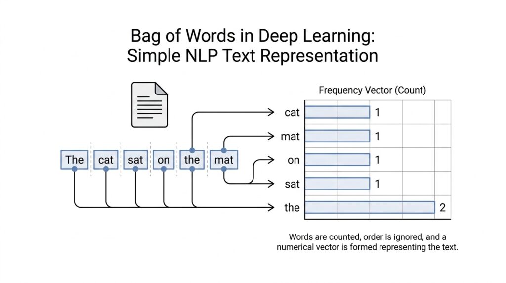
That counting step creates a vector, which is a list of numbers arranged in a fixed order. Each position in the vector belongs to one word in the vocabulary, and the number in that position tells us how often the word appears in the text. So if our vocabulary includes “cat,” “sat,” and “mat,” then a sentence like “the cat sat on the mat” becomes a compact numeric pattern. This is the basic bag of words model: not a story about language, but a scorecard of word presence.
The beauty of this approach is that it is easy to understand and easy to build. We do not need to know grammar, sentence structure, or the deeper meaning of the words to get started. We only need to decide which words belong in the vocabulary and then count them carefully. That simplicity makes bag of words a friendly first step in text representation, especially when we are learning how machines see language as data.
Of course, this simplicity also creates a trade-off, and that trade-off is worth noticing early. Bag of words ignores word order, so “dog bites man” and “man bites dog” can look surprisingly similar if they use the same words. It also misses context, tone, and relationships between nearby words, which means it cannot fully capture meaning the way a human reader does. Still, for many tasks, those raw counts provide enough signal to be useful, especially when we want a fast and understandable baseline.
Another detail that often surprises beginners is that these vectors are usually sparse, which means most positions are zero. If your vocabulary has thousands of words but a single sentence uses only a handful, then most entries stay empty like unused mailboxes in a long row. That might sound wasteful, but it is actually expected and manageable, because the model only needs to notice the few words that are present. From there, we can compare documents, spot patterns, and prepare text for more advanced methods later on.
So at this point, we are not asking language to be elegant; we are asking it to be countable. That is what makes bag of words such a useful starting point in deep learning and other NLP workflows: it gives us a plain, honest numerical snapshot of text. Once we are comfortable with that snapshot, we can move on to richer representations that keep more of the story. For now, the main idea is simple and powerful: in the bag of words model, words become counts, and counts become a form a machine can read.
Prepare the Text
Before we let bag of words start counting, we need to prepare the text so the numbers mean what we think they mean. This is the quiet setup work behind text preprocessing: we decide how to split text into pieces, whether to lowercase it, and how to treat punctuation and accents. If you have ever asked, “How do you prepare text for bag of words?” this is the part where the answer begins. In common implementations such as scikit-learn’s CountVectorizer, lowercasing happens by default, and punctuation is treated as a separator during tokenization.
That matters because the same word can show up in many disguises. “Cat,” “cat,” and “CAT” may look like different tokens unless we normalize them, and accent marks can create another layer of mismatch. CountVectorizer lets you strip accents during preprocessing, which helps keep the vocabulary smaller and cleaner. When we prepare text well, we are not changing the story of the document; we are making sure the same word lands in the same counting bucket every time.
Tokenization is the next doorway. It means splitting a document into tokens, which are small units such as words or word-like pieces, and spaCy describes this as segmenting text into a Doc object that preserves the original text structure. In bag of words, tokenization is where a sentence stops being a sentence and starts becoming a list of countable items. The exact rule matters: scikit-learn’s default pattern keeps tokens of two or more alphanumeric characters, which means punctuation disappears from the counting view.
Once the text is tokenized, we often look at stop words, the very common words that carry little meaning on their own, such as “the” or “and.” Removing them can make a bag of words model focus more on the words that separate one document from another, but the choice is never automatic. Scikit-learn warns that stop word lists need the same preprocessing and tokenization as the vectorizer, or you can end up removing the wrong pieces. That is a useful reminder: text preprocessing works best when every rule matches the rest of the pipeline.
Sometimes we take one more step and compress related word forms together. Stemming is the rougher method: it trims endings so “connecting,” “connected,” and “connection” may land closer together, while lemmatization tries to reduce a word to its dictionary form, or lemma, using language-aware rules. NLTK’s stemmer and WordNet lemmatizer are common examples of these ideas. In a bag of words setup, this can shrink the vocabulary and help similar forms share a count, which is helpful when you want fewer near-duplicate features.
After all of that cleanup, the text is ready to become a matrix row. Scikit-learn’s CountVectorizer turns a collection of documents into token counts and stores them as a sparse matrix, which means it only records the nonzero entries instead of wasting space on every zero. That sparse shape is exactly what we expect after text preparation, because most documents use only a small slice of the full vocabulary. Once the text is clean, tokenized, and consistently handled, the counting step feels much less mysterious, and we can move on with a bag of words representation that is far easier to compare and feed into a model.
Build the Vocabulary
Now that the text has been cleaned and split into tokens, we arrive at the moment where bag of words starts to feel real: we need to build the vocabulary. This is the point where we decide which words deserve a place in our counting system, and that decision shapes everything that follows. If you have ever wondered, how do we build a vocabulary for bag of words?, the answer begins with a simple idea: we collect every unique token we want to track and give each one a fixed slot.
Think of the vocabulary as a shared list of names on a clipboard. Every document in the corpus will be checked against that same list, so the order and size of the vocabulary must stay consistent from start to finish. A word appears once in the vocabulary, even if it shows up a hundred times across the corpus, because the vocabulary is about identity, not frequency. That shared structure is what lets bag of words turn text into a machine-readable vector later on.
The next question is what we include, because not every token should always earn a place. In practice, we often start from the cleaned tokens produced by text preprocessing and then decide whether to keep punctuation-free words, lowercase forms, stop words, or other filtered pieces. This choice matters because the vocabulary is not just a list; it is the lens through which the model will see language. A smaller vocabulary can make the model leaner, while a larger one can preserve more detail, and both choices come with trade-offs.
This is also where CountVectorizer quietly does a lot of the heavy lifting for us. In scikit-learn, CountVectorizer learns the vocabulary from the corpus by scanning the documents, assigning each unique token a stable index, and then using that mapping to build the count matrix. You can think of it like labeling mailboxes before any letters arrive: once the labels exist, every word knows exactly where it belongs. That index mapping is what keeps the bag of words representation organized and repeatable.
Vocabulary building also helps explain why bag of words can feel both powerful and limited. On one hand, it gives us a clean snapshot of the words that appear in our data, which is enough for many simple text classification tasks. On the other hand, the model cannot infer meaning from a word it has never seen, so an unseen token at prediction time has nowhere to go in the vocabulary. That is why we say the vocabulary is the model’s memory of language, but only the part of language it has already met.
Another detail that matters is consistency across training and new text. We usually build the vocabulary on the training corpus first, then reuse the same word-to-index map when we transform new documents later. This keeps the bag of words feature space stable, which means each position in the vector always refers to the same word. Without that stability, our counts would shift around like labels on a moving shelf, and comparison would become unreliable.
There is also a practical side to vocabulary size that beginners notice quickly. A very large vocabulary can make the sparse matrix wider and harder to work with, while a very small one may flatten away useful distinctions between documents. So when we build a vocabulary for bag of words, we are really balancing detail against simplicity. That balance is part of the craft, and it becomes easier to judge once you have seen a few examples in action.
By the time the vocabulary is in place, the rest of the pipeline starts to make sense: every token has a home, every document can be counted against the same list, and every vector has a predictable shape. That is the quiet but essential job of vocabulary building in bag of words and text preprocessing. Once we have that foundation, we are ready to turn those word slots into actual counts and see how the representation comes alive.
Count Word Frequencies
Now that the vocabulary is in place, the next move in bag of words is the part that feels almost mechanical in a reassuring way: we count word frequencies. We take each document, walk through its tokens, and ask how many times each vocabulary word appears. If you have ever wondered, “How do you count word frequencies in a bag of words model?” this is the moment where the whole system clicks, because the abstract idea of text representation turns into a row of numbers we can actually inspect.
The counting step is easier to picture if we think of the vocabulary as a set of labeled bins. Every time a word from the text appears, we drop one token into its matching bin, and the bin’s total becomes that word’s frequency. A word that appears once gets a small value, while a word that repeats over and over leaves a much larger mark. In other words, bag of words does not treat every word equally; it lets repetition speak louder, which is often exactly what we want when we are trying to capture the main themes of a document.
This is where the model starts to reflect emphasis, not just presence. If a product review repeats “great” five times and “slow” once, those frequencies hint at the review’s overall tone without needing any grammar lesson or deep language parsing. That is the power of counting word frequencies: the numbers preserve which words showed up, and they also preserve how strongly each one showed up. For many beginners, this is the first time text representation starts to feel practical rather than theoretical.
A small example makes the process easier to hold in your mind. Suppose our vocabulary includes “cat,” “sat,” and “mat,” and the sentence is “the cat sat on the mat, and the cat stayed.” After preprocessing, the model counts each vocabulary word in order, so “cat” gets 2, “sat” gets 1, and “mat” gets 1. The result is a vector of counts, and that vector becomes the document’s numeric fingerprint inside the bag of words model.
These raw counts matter because they create a consistent scale across documents. One short note might use a word once, while a longer paragraph might use it many times, and the frequency values reveal that difference directly. In practice, this helps us compare documents and spot patterns, especially when we want a simple baseline before moving into more advanced NLP methods. Word frequencies are not trying to be clever; they are trying to be faithful to what the text actually contains.
Of course, the counts can also grow unevenly, and that is something we need to notice. Very common words may appear frequently across many documents, while rare words may appear only once or twice, even if they matter a great deal in context. That imbalance is one reason people sometimes move beyond plain bag of words later on, but the raw counts still give us a solid starting point. They show us the structure of language as data, even when they do not fully explain the meaning behind it.
Another useful detail is that frequency counts are easy to store and compare because they fit naturally into a sparse matrix. Most documents use only a small slice of the vocabulary, so most count positions stay at zero, and the model records only the nonzero values. That makes counting word frequencies both memory-friendly and fast enough for many introductory machine learning tasks. It is one of the reasons bag of words remains such a common first stop in NLP workflows.
So when we count word frequencies, we are doing more than tallying tokens. We are turning a document into a shape the model can read, where repeated words become stronger signals and the vocabulary gives every count a fixed place. That simple act of counting is what gives bag of words its usefulness: it turns language into a measurable pattern, and that pattern is ready for the next step in our journey.
Implement in Python
Now that the idea of bag of words is clear, the real question becomes: how do you implement bag of words in Python without getting lost in details? This is where the concept stops feeling abstract and starts behaving like a tool you can use. Python gives us a few paths, but the most common starting point is CountVectorizer from scikit-learn, a library that turns text into count-based features for machine learning.
The reason CountVectorizer feels so helpful is that it carries the boring-but-important parts for us. It builds the vocabulary, assigns each word a fixed position, and counts how often each word appears in every document. In other words, it gives us a practical bag of words implementation in Python while keeping the workflow readable enough for beginners. If you have been asking yourself, “How do I turn text into numbers in Python?” this is usually the first answer worth learning.
Here is the shape of the process in code. We start with a small collection of documents, feed them into the vectorizer, and then ask for the resulting matrix. The matrix is the numeric version of our text, and each row represents one document from the corpus.
from sklearn.feature_extraction.text import CountVectorizer

texts = [
    "the cat sat on the mat",
    "the dog sat on the log",
    "the cat and the dog"
]

vectorizer = CountVectorizer()
X = vectorizer.fit_transform(texts)

print(vectorizer.get_feature_names_out())
print(X.toarray())
When we run this, fit_transform() does two jobs at once. fit() learns the vocabulary from the training text, and transform() converts each document into counts using that vocabulary. The get_feature_names_out() method shows us the learned words in their exact order, and toarray() converts the sparse matrix into a visible grid so we can inspect it more easily.
That output is the heart of bag of words in Python. Each row becomes a document vector, and each column stands for one vocabulary word such as cat, dog, or sat. If a word appears twice in a document, the corresponding cell gets a 2; if it does not appear at all, the cell stays at 0. This is the same counting logic we talked about earlier, only now it is happening inside code instead of in theory.
Sometimes it helps to see the same idea with a tiny manual version, because that reveals what the library is doing behind the scenes. You can use Python’s built-in Counter from the collections module to count tokens yourself, which is a nice way to understand the mechanics before relying on the library. That approach is slower and less convenient for real projects, but it shows the logic very clearly.
from collections import Counter

vocabulary = ["cat", "dog", "sat"]
document = "cat sat sat"
counts = Counter(document.split())
vector = [counts[word] for word in vocabulary]

print(vector)
This small example shows the same pattern in a more hands-on way. We choose a vocabulary, split the text into tokens, and then count how many times each vocabulary word appears. If you want to understand bag of words in Python from the ground up, this kind of manual check can make the library version feel much less mysterious.
As you start building real examples, preprocessing becomes part of the story again. Lowercasing, removing punctuation, and deciding whether to exclude stop words all affect the final counts, so the vectorizer must see text in the same form every time. If you fit the vocabulary on training data, you should reuse that same fitted vectorizer on new documents later, because changing the vocabulary would scramble the meaning of each column. That consistency is what keeps your bag of words representation stable.
One detail that beginners notice quickly is that the result is usually sparse, meaning most cells are zero. That is normal, because a document only uses a small slice of the full vocabulary. CountVectorizer stores the result efficiently as a sparse matrix, which is a memory-friendly format that only tracks the nonzero values. So when you implement bag of words in Python, you are not just counting words; you are building a structured feature space that can feed into classifiers, clustering models, or anything else that accepts numeric input.
Once you have this working, the rest of the pipeline becomes much easier to follow. You can inspect the vocabulary, compare documents, and experiment with different preprocessing choices to see how the counts change. That is the real payoff of a bag of words implementation in Python: it gives you a simple, visible bridge between raw language and machine learning features, and it does so in a way that is easy to test, tweak, and trust.
Know the Limitations
At this point, bag of words has earned its place as a friendly first model, but we also need to see where it starts to stumble. The limits of bag of words show up the moment you ask it to notice how words work together, not just whether they appear. If you have ever wondered, “Why does bag of words miss the meaning I can feel in a sentence?”, this is the reason: it counts words, but it does not understand the relationships between them.
The first limitation is word order, and it is a big one. Once we turn text into counts, “the dog chased the cat” and “the cat chased the dog” can look almost identical because the same words are present. That is fine when you only need a rough signal, but language is full of small turns that change the whole message, and bag of words tends to flatten those turns into the same pile of counts.
Context creates a second problem, and this one becomes obvious when a word changes meaning depending on its neighbors. A sentence like “The battery died” and “The patient died” uses the same verb, yet the feeling and subject are very different. Bag of words in NLP treats the word “died” the same in both cases, because it does not keep the surrounding words close enough to explain what kind of story is unfolding.
That same weakness shows up with synonyms and multiple meanings. If one writer says “great,” another says “excellent,” and a third says “fantastic,” bag of words may treat them as separate features even though they point in the same direction. It also struggles with words that wear two hats, like “bank,” which can mean a place for money or the side of a river. Without context, the model sees the same token and misses the different roles it can play.
There is also a practical trade-off hiding behind the simplicity: sparse vectors can become very large. As the vocabulary grows, each document still uses only a tiny fraction of those words, so most of the vector stays empty. That sparsity is not a mistake, but it can make the feature space wide, memory-heavy, and a little unwieldy, especially when the corpus grows and the vocabulary keeps expanding.
Another limitation is that raw counts can give too much weight to repetition. If a document repeats one common word many times, that word may dominate the vector even when a rarer word carries more useful information. In other words, bag of words can be loud without being wise; it knows what was repeated, but not whether the repetition matters. This is one reason people often move from plain counts to richer text representation methods later on.
We also have to think about words the model has never seen before. When a new document introduces an unseen token, the vocabulary has no slot for it, so the model cannot count it in the usual way. That means bag of words is tied closely to the training data it has already met, which can make it feel a little brittle when language shifts, new slang appears, or a domain introduces specialized terms.
So what do we do with these limits? We treat them as a map, not a failure. Bag of words is still valuable because it gives us a fast, readable baseline, and that baseline helps us notice when we need something smarter, such as methods that keep order, context, or semantic similarity in view. The important lesson is that bag of words works best when we want a simple snapshot of text, but we should not ask it to solve the full puzzle of language.