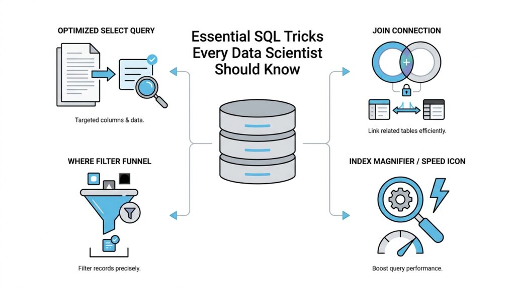
Master Joins and Filters
When you first start stitching tables together, SQL joins can feel a little like trying to match two decks of cards in your head. One table might hold customers, another might hold orders, and your job is to ask SQL to line up the right rows so the story makes sense. That is where joins and filters work together: joins connect the pieces, and filters narrow the scene so you are looking at the rows that matter. If you have ever wondered, “Should this condition go in the join or in the filter?” you are already asking the right question.
A join is the bridge between tables. An INNER JOIN keeps only rows that match on both sides, while a LEFT JOIN keeps everything from the left table and fills in missing matches with NULL, which means no value was found. Think of it like meeting someone at a train station: an inner join says, “Only show me the pairs who both arrived,” while a left join says, “Show me everyone on my list, even if their partner never showed up.” That one idea unlocks a huge amount of SQL joins work for data scientists.
The next move is understanding the difference between the join condition and the filter. The join condition, usually written with ON, tells SQL how rows should match. A filter, usually written with WHERE, tells SQL which rows to keep after the matching happens. That distinction matters because SQL joins and filters do not always behave the same way, especially when NULL values appear.
Here is the simplest version of the pattern:
SELECT c.customer_id, c.name, o.order_id
FROM customers c
LEFT JOIN orders o
  ON c.customer_id = o.customer_id
WHERE c.signup_date >= '2025-01-01';
In this example, the ON clause builds the relationship between customers and orders, while the WHERE clause filters the customers we want to study. The result is easy to reason about because each part has one job. Once you separate those jobs in your mind, joins and filters stop feeling tangled and start feeling like a clean two-step process.
A small twist appears when you filter the table on the right side of a left join. If you place that filter in WHERE, you may accidentally remove the rows you hoped to preserve, because WHERE runs after the join has already produced NULLs for missing matches. What is the practical lesson here? If you want to keep unmatched rows from the left table, put the right-table condition in the ON clause instead of the WHERE clause. That one habit can save you from a very common SQL surprise.
For example, imagine you want customers and only their completed orders. If you write the completed-order rule inside ON, the left join still keeps customers with no completed orders, and their order columns stay NULL. If you move that same rule into WHERE, you filter those NULL rows away and the query starts acting more like an inner join. This is one of those details that feels tricky at first, but once you see it, the logic becomes much easier to trust.
The final skill is learning to combine filters without losing your place. AND narrows the result set by requiring every condition to be true, while OR broadens it by allowing any condition to match. When you layer those conditions carefully, SQL joins and filters become a precise tool for answering business questions, not just a way to fetch rows. And as you keep practicing, you will start reading queries the way a detective reads clues: the join tells you who belongs together, and the filter tells you which parts of the story deserve your attention.
Simplify Queries With CTEs
When a query starts to feel like a stack of sticky notes, CTEs, or Common Table Expressions, give you a place to lay each note out in order. A CTE is a named temporary result set that lives only inside a single SQL statement, and you can refer to it later in that same statement, even more than once. That makes it a perfect companion to the joins and filters you’ve already been working with, because it lets you break one large question into smaller, readable steps.
How do you keep a query readable when it starts to sprawl? You name the pieces. Instead of burying a filter inside a join inside another filter, you can write the logic in stages so each step has a clear job. First, you narrow the data. Then you connect it. Then you ask the final question. That rhythm feels a lot like preparing ingredients before cooking: once each part is in its own bowl, the whole recipe becomes easier to follow.
Here is the shape of that idea in SQL:
WITH recent_orders AS (
  SELECT order_id, customer_id, order_total
  FROM orders
  WHERE order_date >= '2025-01-01'
),
active_customers AS (
  SELECT customer_id, name
  FROM customers
  WHERE signup_date >= '2025-01-01'
)
SELECT c.name, r.order_id, r.order_total
FROM active_customers c
LEFT JOIN recent_orders r
  ON c.customer_id = r.customer_id;
This query tells a story in three scenes. The first CTE collects the orders we care about, the second CTE collects the customers we care about, and the final SELECT brings them together with a join. Because each CTE has a name, you can read the query almost like a paragraph: one part prepares recent orders, another part prepares active customers, and the last part combines them. That is the real gift of CTEs in SQL: they turn a dense block of logic into a sequence you can reason through.
CTEs also help when the same intermediate result appears more than once. If you need a filtered dataset in two different joins or calculations, a CTE lets you define it once and reuse it instead of repeating the same subquery. That reduces copy-paste mistakes and makes later edits safer, because you only change the logic in one place. In practice, that means less hunting through nested parentheses and more confidence that every branch of the query is using the same definition.
Another quiet advantage is that CTEs give you a cleaner mental model than deeply nested subqueries. A subquery hides its work inside another statement, while a CTE puts the work up front, where you can name it and inspect it more easily. That does not mean CTEs are always faster; it means they are often easier to understand, which matters a lot when you are debugging a tricky analysis at the end of a long day. If you have ever asked, “What does this middle step actually contain?” a CTE is the SQL answer to that question.
Once you get comfortable, CTEs can do one more elegant trick: they can reference themselves in a recursive CTE, which is a CTE that repeatedly feeds its own output back into the query. That pattern is useful for tree-like data such as org charts, folder structures, or category hierarchies, where one row leads to the next. Even if you are not using recursion yet, it helps to know the door is there. For now, the main habit is simple: when a query starts to blur together, pause, name the intermediate steps, and let CTEs carry the weight for you.
Rank Rows Using Window Functions
Now that we can cleanly shape a dataset with joins and CTEs, we can do something that feels almost magical: we can rank rows using window functions without collapsing the table. A window function is a SQL function that looks across a small “window” of related rows while still keeping each row visible in the output. That matters when you want to compare records inside the same group, like finding the top sale for each customer, the newest event for each user, or the best-performing product in each category. If you have ever wondered, “How do I rank rows in SQL without losing the detail?” this is the move that answers it.
The idea is easier to picture if you imagine each group standing in its own line. A partition means the group you want to analyze, such as one customer, one store, or one category. An ORDER BY inside the window tells SQL how to line up the rows inside that group, usually from newest to oldest, largest to smallest, or best to worst. Together, PARTITION BY and ORDER BY tell SQL where each little ranking contest begins and how the finish order should look. You are not sorting the whole table into one pile; you are creating many small races at once.
Here is the pattern in action:
SELECT
  customer_id,
  order_id,
  order_total,
  ROW_NUMBER() OVER (
    PARTITION BY customer_id
    ORDER BY order_total DESC
  ) AS order_rank
FROM orders;
This query gives every order a position within its customer’s group. The largest order gets rank 1, the next largest gets rank 2, and so on. ROW_NUMBER() means “assign a unique sequence number,” so even if two orders tie, each one still gets a different number. That makes it a reliable choice when you need one clear winner per group, such as the single most recent session or the single highest purchase.
The story gets more interesting when ties appear, because not every ranking function handles them the same way. RANK() gives tied rows the same position, but it leaves a gap after the tie, like two runners sharing second place and then jumping to fourth. DENSE_RANK() also gives ties the same position, but it does not leave gaps, so the next row becomes third instead of fourth. Those differences sound small, but they change the answer in ways that matter when you are reporting leaders, tiers, or top-N results. Choosing the right ranking function is less about memorizing names and more about deciding how you want ties to feel in the story.
That choice becomes especially useful when you only want the top row in each group. Suppose you need the highest-value order per customer or the newest record per user. You can wrap the ranking query in a CTE, then filter for order_rank = 1, which keeps the first row from each partition and leaves the rest behind. In other words, window functions let you prepare the ranking first, and then you can filter with the same calm structure you already used for joins and CTEs. The result is a query that reads like a sequence of decisions instead of a maze of nested logic.
The real power of SQL window functions is that they let you rank rows and still keep the full dataset intact for later analysis. That means you can sort, compare, and flag records without losing the surrounding context that often matters just as much as the winner itself. Once you get comfortable with row numbers, ranks, and dense ranks, you start seeing them everywhere: leaderboards, deduping records, session analysis, funnel steps, and “top 3 per group” questions. And as we move forward, that same windowing pattern will keep showing up as one of the most flexible tools in your SQL toolkit.
Filter Results With Subqueries
Sometimes the cleanest way to answer a question in SQL is to ask a smaller question first. That is the heart of SQL subqueries: you filter results by nesting one query inside another, letting the inner query gather a clue before the outer query makes the final decision. If joins felt like connecting tables and CTEs felt like laying out the steps in order, subqueries feel like whispering, “Hold on—let me check one thing before we continue.” What if you only want customers who spent more than the average customer? This is where subqueries in SQL become a quiet but powerful tool.
The simplest version is a scalar subquery, which means a subquery that returns a single value. You can think of it like a tiny calculator tucked inside your WHERE clause. Instead of hardcoding a number, you let SQL compute the threshold for you, which keeps the query tied to the data itself. That makes your filter more flexible and more honest, especially when the underlying numbers change every day.
SELECT customer_id, order_total
FROM orders
WHERE order_total > (
  SELECT AVG(order_total)
  FROM orders
);
Here, the inner query finds the average order total, and the outer query keeps only the rows above that average. The logic reads like a conversation: first, discover the benchmark; then, keep the rows that clear it. This is one of the most common ways to filter results with subqueries, because it turns a vague idea like “above average” into something SQL can measure precisely.
Subqueries become even more useful when you want to filter by membership in a set of values. In that case, IN lets the outer query check whether a value appears in the list returned by the inner query. Imagine you want customers who placed at least one order in a specific month, or products that belong to categories with strong sales. The subquery gathers the qualifying IDs, and the outer query uses them as a filter.
SELECT customer_id, name
FROM customers
WHERE customer_id IN (
  SELECT customer_id
  FROM orders
  WHERE order_date >= '2025-01-01'
);
This pattern is easy to read because the inner query defines the group first and the outer query fetches the matching rows afterward. If you’ve ever asked, “How do I filter rows based on another query in SQL?” this is one of the first answers worth learning. It feels a little like making a guest list from one notebook and then checking names at the door with another.
Another useful pattern is EXISTS, which asks whether the subquery finds at least one matching row. Unlike IN, which cares about a list of values, EXISTS cares about whether a related record is present at all. That makes it especially handy when you want to filter out rows that have no matching activity, no linked event, or no supporting record. In plain language, EXISTS says, “Show me the row if the answer to this smaller question is yes.”
Correlated subqueries take that idea one step further by letting the inner query refer back to the current row from the outer query. That sounds intimidating, but the mental model is simple: for each row in the outer query, SQL runs a tiny check using that row’s values. You might use this to find customers whose order exceeds their own average, or products whose price beats the average in their category. The subquery and the outer query work together like a lock and key, with each row supplying the context the inner query needs.
SELECT o1.customer_id, o1.order_id, o1.order_total
FROM orders o1
WHERE o1.order_total > (
  SELECT AVG(o2.order_total)
  FROM orders o2
  WHERE o2.customer_id = o1.customer_id
);
This query keeps orders that are above each customer’s own average, not the average for the whole table. That distinction matters because it lets you compare rows against the right reference point. A global benchmark and a row-level benchmark can tell very different stories, and correlated subqueries help you choose the one that matches your question.
The real skill is knowing when a subquery is the clearest way to filter results and when a CTE or join will read more naturally. Subqueries in SQL shine when the logic is compact, the check is self-contained, and you want the outer query to stay focused on the final result. As you practice, you’ll start to feel when the question inside the question makes the whole query easier to think about, and that is when filtering with subqueries stops feeling tricky and starts feeling like one more tool you can trust.
Aggregate Data With CASE
You’ve already seen how SQL can connect tables, narrow rows, and even rank records without losing detail. Now we arrive at a very handy next step: using CASE to turn raw rows into summaries that answer a specific question. If you have ever wondered, “How do I count orders by status in SQL without writing a separate query for each one?” conditional aggregation is the pattern that makes the answer feel natural. It lets you keep one table of events and still pull out clean totals for each situation.
The key idea is that CASE works like a decision point inside a query. A CASE expression checks a condition and returns one value when the condition is true and another when it is false, which makes it perfect for SQL aggregate functions such as COUNT, SUM, and AVG. Think of it like sorting mail into different bins before you count the envelopes in each bin. Instead of building several filtered queries, we let one query make the decisions row by row and then aggregate the results.
That pattern becomes especially useful when your data has statuses, categories, or flags. Maybe you want to know how many orders were completed, how many were canceled, and how many are still pending. Rather than running three separate queries, you can ask SQL to evaluate each row and then add up the answers. This is what people usually mean when they talk about aggregate data with CASE.
Here is the basic shape of the pattern:
SELECT
  COUNT(*) AS total_orders,
  SUM(CASE WHEN status = 'completed' THEN 1 ELSE 0 END) AS completed_orders,
  SUM(CASE WHEN status = 'canceled' THEN 1 ELSE 0 END) AS canceled_orders,
  SUM(CASE WHEN status = 'pending' THEN 1 ELSE 0 END) AS pending_orders
FROM orders;
Each row in orders passes through the CASE expression like a checkpoint. If the status matches, SQL returns 1; if it does not, SQL returns 0. Then SUM adds those tiny signals together, giving us a count for each category. The query stays compact, but the result reads like a small dashboard.
A common question is: why not use COUNT everywhere? The answer is that COUNT and SUM solve slightly different versions of the same problem. COUNT(CASE WHEN ... THEN 1 END) works well because COUNT ignores NULL, while SUM(CASE WHEN ... THEN 1 ELSE 0 END) makes the logic very explicit by turning every row into either a one or a zero. Both are valid forms of conditional aggregation in SQL, and the clearer one is often the better choice when you are still building confidence.
The real strength of this technique shows up when you group by something else, like customer, month, or region. You can ask for one summary row per customer and still include several conditional counts in the same result. That means you can see, for example, how many completed orders each customer placed, how many were refunded, and how many were still open. Instead of stacking separate reports on top of one another, you let SQL build a multi-column summary in one pass.
SELECT
  customer_id,
  SUM(CASE WHEN status = 'completed' THEN 1 ELSE 0 END) AS completed_orders,
  SUM(CASE WHEN status = 'refunded' THEN 1 ELSE 0 END) AS refunded_orders
FROM orders
GROUP BY customer_id;
This is one of those SQL tricks that feels small at first and then starts appearing everywhere. You can use it for quality checks, funnel analysis, category comparisons, and any reporting task where one dataset needs to answer several related questions at once. As you practice, you’ll start to see that CASE does not replace aggregation; it gives aggregation a memory, so the final summary can distinguish one kind of row from another. That is the trick that turns a flat table into a story you can actually read.
Speed Up Slow Queries
When a query that used to feel snappy starts dragging, the first instinct is usually to stare at the wrong place. You may have only asked for a few rows, so why is SQL working so hard? The answer often lives in query performance: the database is doing extra work somewhere, and our job is to make that path shorter, simpler, and more direct. If you are trying to speed up slow queries, the most helpful habit is to think like the database does, one step at a time.
The quickest win is to reduce the amount of data SQL has to touch. That means filtering early, selecting only the columns you need, and avoiding the urge to carry every field through every step of the query. A database reads data from disk and memory in chunks, so every extra row and every extra column adds weight. When we keep the result shape lean, we make slow SQL queries less likely before they ever become a problem.
Indexes are the next character in the story. An index is a separate data structure that helps the database find rows faster, a little like the index in the back of a book that points you to the right page instead of making you read every chapter. Columns you use often in joins, filters, and sorting are the usual candidates. If your query keeps searching by customer_id or order_date, an index on those columns can dramatically improve query performance because SQL can jump to the relevant rows instead of scanning the whole table.
That said, indexes only help when the database can use them clearly. If you wrap an indexed column inside a function, like DATE(order_date) or LOWER(email), the engine may have to work harder because it can no longer match the raw index as easily. What does that mean in practice? Instead of asking SQL to transform every row before filtering, try to compare the column in its original form whenever you can. This small change is one of the most common answers to the question, “Why is my SQL query slow even though I have an index?”
Joins deserve a careful look too, especially because we have already seen how powerful they can be. A join becomes expensive when it matches far more rows than you expected, or when you join before trimming the data down to size. One useful pattern is to aggregate or filter each side first, then join the smaller results. That reduces the amount of work the database has to do, and it often makes a slow query feel much lighter. In other words, do not ask SQL to carry a crowd across the bridge if only a few people need to cross.
CTEs, or Common Table Expressions, can help you organize that thinking, but they are not a magic speed button. A CTE is a named temporary result set, and it makes logic easier to read, yet some databases may still treat it like a separate step that gets computed before the final query. That is why the fastest-looking version and the clearest version are not always the same thing. When you want to speed up slow queries, it helps to test whether a CTE, subquery, or inline join gives your database the easiest route, not just the prettiest shape.
At this point, the most valuable tool is the execution plan, which is the database’s roadmap for how it intends to run your query. An execution plan shows whether SQL is scanning a whole table, using an index, sorting a large result, or joining data in a costly way. You do not need to become an engine mechanic to benefit from it; you only need to notice the big clues, like a full table scan on a huge dataset or a sort happening much earlier than expected. Once you can read that roadmap, query performance stops feeling mysterious and starts feeling diagnosable.
The final habit is to remove repeated work wherever possible. If a query calculates the same filtered subset again and again, or ranks the same rows several times, it may be worth materializing that step outside the main query or reusing a cleaned intermediate result. That is where the earlier tools begin to connect: joins become smaller, filters become earlier, and summaries happen before expensive comparisons. The result is not just faster SQL, but SQL that tells the database exactly where to spend its energy.