Pick the 1.5B Base Model
Before we touched training settings, we had to answer a more human question: which 1.5B base model should carry the project? That choice mattered more than it first seemed, because QLoRA keeps the pretrained weights frozen and learns task-specific changes through small LoRA adapters on top of a 4-bit quantized base model. So the base model is not the whole story; it is the foundation we build on, and a good foundation makes the later fine-tuning feel steady instead of fragile.
We wanted a model that was compact enough to fine-tune comfortably, but still strong enough to learn the behaviors we cared about. Qwen2.5-1.5B is a good example of that balance: the base model has 1.54 billion parameters, a 32,768-token context window, and multilingual coverage across 29+ languages. That means you are not starting from a tiny toy model, but from a small language model that already has enough breadth to make QLoRA training worth the effort.
Another reason we leaned toward a base model instead of an instruction-tuned one is that the model card frames the base checkpoint as something to post-train further with methods like supervised fine-tuning. That fit our plan exactly, because we wanted to teach the model our task and our output style without inheriting someone else’s conversational habits too early. If you are asking, “Which 1.5B base model should I pick for QLoRA fine-tuning?”, the best answer starts with alignment: does the checkpoint already match your language, context length, and deployment needs?
We also paid attention to the pieces beginners often overlook, like tokenizer fit and context length. A 32k-token window matters because it lets us keep longer examples intact instead of chopping every sample into awkward fragments, and that usually makes the learning signal cleaner. It is a little like setting out fabric on a wide table instead of a tiny desk: when you have room, you cut fewer pieces in the wrong places, and the final shape comes together more naturally.
The smaller parameter count was the practical advantage that tied everything together. A 1.5B model gives QLoRA more breathing room on modest hardware, since the frozen weights stay compressed while the adapters carry the learning burden. That matters when you want to iterate quickly, compare runs, and avoid spending your day fighting memory spikes instead of improving the fine-tuning recipe. In a project like this, the 1.5B base model is not a compromise; it is what gives you enough speed and headroom to experiment well.
In the end, the base model choice was less about chasing a famous name and more about finding the right working partner for the job. We wanted a 1.5B base model that already spoke fluent language, had enough context to handle our data, and left room for QLoRA to do its quiet, efficient work. Once that foundation was in place, the rest of the pipeline could focus on teaching behavior instead of compensating for a weak starting point.
Prepare Clean Training Data
Once the base model is chosen, the next real challenge is the training data, because QLoRA fine-tuning lives or dies on what we feed it. If you are wondering, “What does clean training data actually look like?” the answer starts with a simple idea: fewer, better examples often beat a larger pile of messy ones. Recent work on supervised fine-tuning also points in the same direction, showing that data quality can matter more than raw quantity, and that small high-quality datasets can still produce strong results.
So we began by turning raw examples into a single, predictable shape. Each sample needed the same structure, whether that was a prompt/completion pair or another format we had chosen, so the model would not have to guess where the question ended and the answer began. That consistency matters because the model is learning a pattern, not reading a spreadsheet, and every bit of format drift adds noise to that pattern. In practice, clean training data feels a lot like arranging ingredients before cooking: once everything sits in the right bowl, the rest of the process stops feeling chaotic.
After that, we removed duplicates, near-duplicates, and contradictory examples, which is the data version of hearing the same sentence repeated in three different voices. A duplicate is the same example copied again, while a near-duplicate is a case that looks almost identical but adds no new information. That cleanup is worth the effort because low-value patterns can be redundant, uninformative, or even harmful during supervised fine-tuning, and continuing to train on them can drag down downstream performance.
We also checked for label hygiene, meaning we made sure the answers matched the task we wanted the model to learn. If one example teaches the model to be concise and the next one rewards rambling, the training signal starts to wobble, and the model learns uncertainty instead of style. This is where a clean training set earns its keep: it gives QLoRA a clear, repeatable lesson rather than a stack of mixed messages. The QLoRA paper’s results on small high-quality datasets are a good reminder that clarity in the data can do a lot of heavy lifting.
Then we split the data carefully into training and validation sets. The training set is the material the model actually learns from, while the validation set is a small holdout set we use to check whether it is improving or just memorizing. We kept examples from the same source or family together when needed, because letting closely related examples leak across splits can make the model look better than it really is. That kind of honesty is important: we wanted a model that could generalize in the real world, not one that only looked polished inside the notebook.
The final pass was the human one, and it mattered more than it sounds. We read samples aloud, looked for awkward phrasing, checked whether the task instructions were unambiguous, and asked whether a beginner would understand what the model was supposed to do from that one example alone. That review catches the tiny problems that automated filters miss, like a polite but vague answer, a missing field, or an example that technically works but teaches the wrong habit. When the dataset feels calm and coherent to us, QLoRA has a much easier job learning from it.
By the time we finished, the training data no longer felt like a heap of raw material; it felt like a carefully edited conversation. That difference is easy to overlook, but it is often the gap between a model that merely trains and a model that starts to sound dependable. From here, the next step was making that clean data fit the training pipeline without wasting tokens or memory.
Load QLoRA in 4-Bit
With the dataset cleaned, we finally arrived at the part where QLoRA in 4-bit stops feeling abstract and starts feeling engineered. This is where we load the 1.5B base model with bitsandbytes 4-bit quantization, keep the pretrained weights frozen, and let small LoRA adapters carry the learning. If you’ve been asking, “How do I load a model in 4-bit for QLoRA without running out of memory?”, this is the moment where the answer becomes concrete.
The first choice is the quantization recipe, and that recipe matters more than the name sounds like it should. In the QLoRA paper, the core idea is to backpropagate through a frozen, 4-bit quantized base model, while the Hugging Face docs recommend NormalFloat 4, or NF4, for training 4-bit base models because it is designed for weights that follow a normal distribution. We also turned on double quantization, which compresses the quantization constants themselves and saves more memory, and we used bfloat16, or BF16, as the compute type so the model could do its math a little faster without giving up the 4-bit storage win.
This is what the loading step looked like in practice:
import torch
from transformers import AutoModelForCausalLM, BitsAndBytesConfig
from peft import prepare_model_for_kbit_training

quantization_config = BitsAndBytesConfig(
    load_in_4bit=True,
    bnb_4bit_quant_type='nf4',
    bnb_4bit_compute_dtype=torch.bfloat16,
    bnb_4bit_use_double_quant=True,
)

model = AutoModelForCausalLM.from_pretrained(
    model_id,
    quantization_config=quantization_config,
)

model = prepare_model_for_kbit_training(model)
That tiny block does a lot of heavy lifting. BitsAndBytesConfig tells Transformers to load the model in 4-bit mode, nf4 chooses the QLoRA-friendly quantization format, and bnb_4bit_use_double_quant=True adds the nested quantization step that squeezes memory a bit further. Then prepare_model_for_kbit_training() gets the model ready for adapter training by casting layer norms to fp32, making the output embedding layer trainable, upcasting the lm head to fp32, and optionally enabling gradient checkpointing, which saves memory by trading away some backward-pass speed.
One detail that is easy to miss is that 4-bit loading is not a free pass to fine-tune every weight in the network. The Transformers docs are explicit that 8-bit and 4-bit training is only supported for training extra parameters, which is exactly why QLoRA works so well: the frozen base model stays compressed, and the adapters learn the task-specific changes on top. In other words, we are not asking the whole model to move; we are asking a much smaller set of weights to learn the new behavior.
That distinction changes how the whole pipeline feels. Instead of spending our GPU budget on full-precision model weights, we spend it on useful training signals, cleaner batches, and longer experiments. In a 1.5B model setup, that usually means fewer memory spikes, smoother iteration, and more room to test different adapter settings without constantly reshuffling the hardware plan.
By the time the model is loaded this way, the training stack feels much calmer: the base model sits quietly in 4-bit form, the adapters are ready to learn, and the remaining steps can focus on behavior rather than on memory firefighting. That is the real strength of QLoRA in 4-bit—it gives us a small, disciplined place where the model can grow without pretending the whole network needs to change at once.
Set LoRA Target Modules
Now that the base model is loaded in 4-bit, the next question becomes wonderfully specific: where, exactly, should the LoRA adapters attach? That is what LoRA target modules means in practice. We are not training the whole network; we are choosing the small set of internal layers where the adapters will sit, like adding new hinges to a few important doors instead of rebuilding the whole house. In QLoRA fine-tuning, that choice matters because it shapes how much the model can learn, how much memory we spend, and how naturally the adapters can steer the model’s behavior.
If you are wondering, “Which LoRA target modules should I choose for fine-tuning?”, the safest answer is to start with the parts of the transformer that move information around. In decoder-only language models, those are usually the attention projection layers, often named q_proj, k_proj, v_proj, and o_proj. The q_proj layer makes the query, the k_proj layer makes the key, the v_proj layer makes the value, and the o_proj layer blends the result back into the stream. That sounds abstract at first, but the picture is simple: these layers decide what the model notices, what it connects, and what it passes forward.
We began there because attention layers often give the best balance between flexibility and efficiency. They let QLoRA fine-tuning adjust how the model focuses on context without forcing every weight in the network to change. In a small 1.5B model, that is especially important, because we want the adapters to carry meaningful learning while the frozen 4-bit base model stays stable. You can think of it like teaching someone to read a room better rather than retraining their entire memory of language.
From there, we looked at the feed-forward or MLP layers, which are the parts that transform information after attention has gathered it. These often appear as gate_proj, up_proj, and down_proj in many modern architectures. Adding LoRA to these modules increases adapter capacity, which can help when the task needs more style control, more domain adaptation, or more deliberate output behavior. The tradeoff is that every extra target module adds parameters and memory use, so QLoRA stops feeling lightweight if we attach adapters everywhere without a clear reason.
That is why the choice is less about copying a universal recipe and more about reading the model’s architecture with care. In practice, we usually start small, using the attention projections first, then expand to the MLP projections only if the model needs more room to learn. This staged approach makes LoRA target modules feel less like a guessing game and more like a conversation with the model: we listen to where it struggles, then give it help in the places that matter most. For many fine-tuning jobs, that restraint produces cleaner results than trying to touch every possible layer.
It also helps to match the target modules to the goal of the project. If you are teaching a model a new writing style, attention-only LoRA may be enough because style often depends on how the model organizes context and response flow. If you are pushing the model into a more specialized domain, like technical language or structured outputs, adding MLP layers can give it extra room to reshape internal representations. The key is to treat LoRA target modules as a dial, not a switch: we turn it only as far as the task asks us to.
Once the adapters are placed, the rest of the training recipe becomes easier to reason about. We can decide how much capacity to give those adapters, how aggressively to train them, and whether the model needs a wider or narrower adaptation path. That is the quiet logic behind QLoRA fine-tuning: first we choose the right foundation, then we choose the right places to let it learn, and only after that do we worry about how hard to push.
Tune Training and Memory Settings
At this point, the model is loaded and the adapters are attached, but the real question is whether the run will fit comfortably on the GPU. How do you tune QLoRA training settings without running out of memory? We treated the first pass like packing a small suitcase: keep per_device_train_batch_size small, then use gradient accumulation, which spreads one update across several mini-batches and gives you a larger effective batch size without forcing every example to sit in memory at once. Hugging Face notes that the effective batch size is the per-device batch size multiplied by gradient_accumulation_steps, so a tiny local batch can still behave like a much steadier training run.
Next, we looked at sequence length, which is the number of tokens the model reads in one go. That matters because activations, the temporary values the model saves while it is processing input, scale with both batch size and sequence length. Gradient checkpointing keeps only a few checkpoints and recomputes the rest during backpropagation, so we trade some speed for a much smaller memory footprint; Hugging Face also recommends pairing it with gradient accumulation when memory is tight. This is one of those settings that feels awkward the first time you meet it, then suddenly makes the whole QLoRA training loop feel possible.
For the math itself, we leaned on bfloat16, usually shortened to BF16, which is a 16-bit number format that keeps the model’s calculations fast without pushing everything into full precision. In the 4-bit loading stack, Bitsandbytes documents BF16 as the compute type for 4-bit models, while the QLoRA paper highlights NF4, or NormalFloat 4, and double quantization as the pieces that keep the stored weights compact. Put together, those choices let the frozen base model stay light while the training step still has enough numerical room to learn cleanly.
The hidden memory thief is often the optimizer state, meaning the extra numbers the optimizer keeps so it can update weights well. QLoRA introduces paged optimizers to smooth out memory spikes, and Bitsandbytes provides paged optimizer variants that can move state page-by-page between GPU and CPU. If you’ve ever watched a run fail only when it was almost done, this is the kind of setting that turns a brittle experiment into a stable one.
We also kept the tuning process conservative because 4-bit and 8-bit training only supports training extra parameters, not the quantized base weights themselves. That limitation is actually a gift: it tells you where to spend your effort. Instead of changing everything at once, we tested one lever at a time – batch size, then accumulation steps, then checkpointing, then optimizer choice – so we could see which change reduced memory and which one still left the model learning at a good pace.
Once the first stable run finished, we used the logs to decide whether to widen the batch, lengthen the sequence, or keep checkpointing on. That slow, careful loop is what makes QLoRA training feel practical on modest hardware, because the goal is not to squeeze every last byte out of the GPU; the goal is to give the adapters enough room to learn without letting memory pressure steal the experiment. When the settings are tuned well, the model spends its energy improving instead of merely surviving.
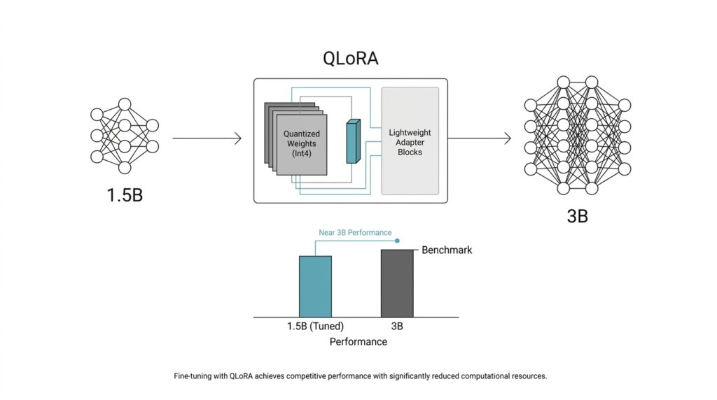
Benchmark Against the 3B Model
Once the 1.5B run was behaving reliably, we had to answer the question that really mattered: how do you benchmark a 1.5B QLoRA model against a 3B model without fooling ourselves? We treated the 3B model as a yardstick, not a trophy, and we ran both models through the same evaluation path so the comparison stayed fair. In Hugging Face’s evaluation tooling, the basic idea is to compare a model, a dataset, and a metric as one unit, which is exactly the kind of structure you want when two models are being judged side by side.
The first rule was consistency. If one model gets a friendlier prompt, a different decoding setup, or a looser scoring rule, the benchmark stops being a comparison and turns into a moving target. That matters because benchmark performance is highly sensitive to the prompt and evaluation setting, and standardized setups are often less flattering than the handcrafted prompt that makes one model shine. So we kept the test conditions aligned and let the numbers speak in the same language for both models.
From there, we looked at the scorecard in layers instead of chasing one magic number. For structured tasks, we used task-specific metrics such as exact match or F1, which measure whether the model hit the answer precisely or recovered the right meaning even when the wording shifted. Hugging Face’s evaluation docs also support bootstrapped confidence intervals, which is useful when you do not want to overreact to tiny score differences that may just be noise. That gave us a cleaner read on whether the 1.5B fine-tuned model was truly closing the gap or merely having a lucky run.
Then we did the part that numbers alone can’t replace: we read the outputs like a person would. A benchmark can tell you whether the answer is technically right, but it cannot always tell you whether the answer feels usable, concise, or aligned with the task’s tone. So we placed the 1.5B output next to the 3B output and asked a very practical question: which one would we actually want to hand to a user? That side-by-side review often revealed the real tradeoff, such as the smaller model being slightly less polished but more consistent in the format we wanted.
We also paid attention to speed and footprint, because a benchmark against a 3B model should measure more than accuracy alone. If the 1.5B QLoRA model gets within reach of the larger model while staying lighter, faster, and easier to deploy, that is part of the win. In other words, the goal was not to prove that smaller is always better; it was to see whether the smaller model earned its place by delivering enough quality for a much lower operational cost.
By the end of the comparison, the 3B model had done its job: it gave us a hard target, a reality check, and a way to see where the 1.5B model still needed help. That kind of benchmark is most useful when it feels honest rather than heroic, because honest comparisons show you both the gains you’ve made and the edge cases you still need to fix.