Loading Sentiment Dataset
Before we can teach a decision tree to recognize tone, we need to meet the raw material it will learn from. That usually means loading the sentiment dataset into memory and turning it from a file on disk into something we can inspect, question, and shape. If you have ever opened a spreadsheet and wondered, “What exactly is inside this file, and how do I get it ready for sentiment analysis?”, you are already standing at the right doorway.
Most sentiment analysis projects begin with a file that stores text and labels side by side. A label is the answer we want the model to learn, such as positive or negative, and the text is the message the model must study to reach that answer. The file is often a CSV, which means comma-separated values, a plain-text table format where each row is one example and each column holds one piece of information. Once we load that file, we usually place it into a DataFrame, a table-like structure that lets us filter, count, clean, and inspect rows without losing our place.
Here is the kind of loading step that usually starts the journey:
import pandas as pd

df = pd.read_csv("sentiment_data.csv")
print(df.head())
This tiny block does a lot of heavy lifting. It brings the sentiment dataset into a DataFrame called df, then shows the first few rows so we can confirm the file opened correctly. When you are new to data science, that first glance matters more than it seems, because it tells you whether the columns look sensible, whether the text appears intact, and whether the labels are where you expect them to be. In a decision tree workflow, this is the moment where the raw data becomes something we can actually reason about.
Of course, real files are rarely perfectly tidy, and that is where the careful part begins. Sometimes the dataset includes a review or text column for the message itself and a sentiment or label column for the class we want to predict. Other times the column names are less obvious, or the file uses a different separator, such as tabs instead of commas. If the text contains special characters, we may also need to pay attention to encoding, which is the way a file stores letters and symbols so they can be read correctly by the computer.
When we load sentiment data, we are not only opening a file; we are checking whether the story inside the file makes sense. Does each row contain one opinion? Are the labels consistent, or do we see variations like pos, positive, and 1 all mixed together? Are there missing entries that might confuse the decision tree later on? These questions matter because a model learns patterns from what we give it, and messy input can lead to noisy predictions. That is why the loading step is really the first quality check in sentiment analysis, not just a mechanical setup task.
If the dataset comes from a common source like a spreadsheet, a CSV export, or a text dataset from a machine learning library, the overall idea stays the same: we bring it into a usable table, then inspect its shape and meaning. A quick look at the number of rows and columns tells us how much training material we have, while a peek at the label counts tells us whether the classes are balanced. That balance matters because a decision tree can be tempted to favor the majority class if one label appears far more often than the other.
So as we load the sentiment dataset, we are doing more than starting the code. We are setting the foundation for everything that comes next: cleaning the text, separating words from labels, and preparing the data for the decision tree to learn from. Once this table is in place, the rest of the workflow starts to feel much more concrete, because now we can see exactly what the model will be asked to understand.
Cleaning Text Data
Now that the raw sentiment dataset is sitting in a DataFrame, the next job is to turn the messy human language inside it into something a decision tree can understand. This is where cleaning text data enters the story, and it matters more than many beginners expect. A machine learning model does not read emotion the way we do; it looks for patterns, so we need to remove noise and keep the words that actually carry meaning. If you have ever asked, “How do I clean text data for sentiment analysis without breaking the meaning?”, you are asking exactly the right question.
The first thing we usually do is make the text consistent. One review may say “Amazing,” another may say “amazing,” and a third may shout “AMAZING!!!” Even though a person sees the same feeling in all three, a computer sees three different versions unless we guide it. So we often convert text to lowercase, remove extra spaces, and strip punctuation that does not help the model learn. In sentiment analysis, this step feels like putting scattered puzzle pieces into the same box so we can sort them more easily.
From there, we start clearing away the small distractions that clutter the message. These distractions can include HTML tags, digits, emojis, and symbols that appear in the raw data but do not help with the label we want to predict. For example, a review like “
Great movie!!! 10/10” contains useful praise, but the tag and numbers may not add much value for a decision tree. At the same time, we have to be careful not to scrub too aggressively, because every cleanup choice changes the story the model sees. The goal is not to make the text pretty; the goal is to make it useful.
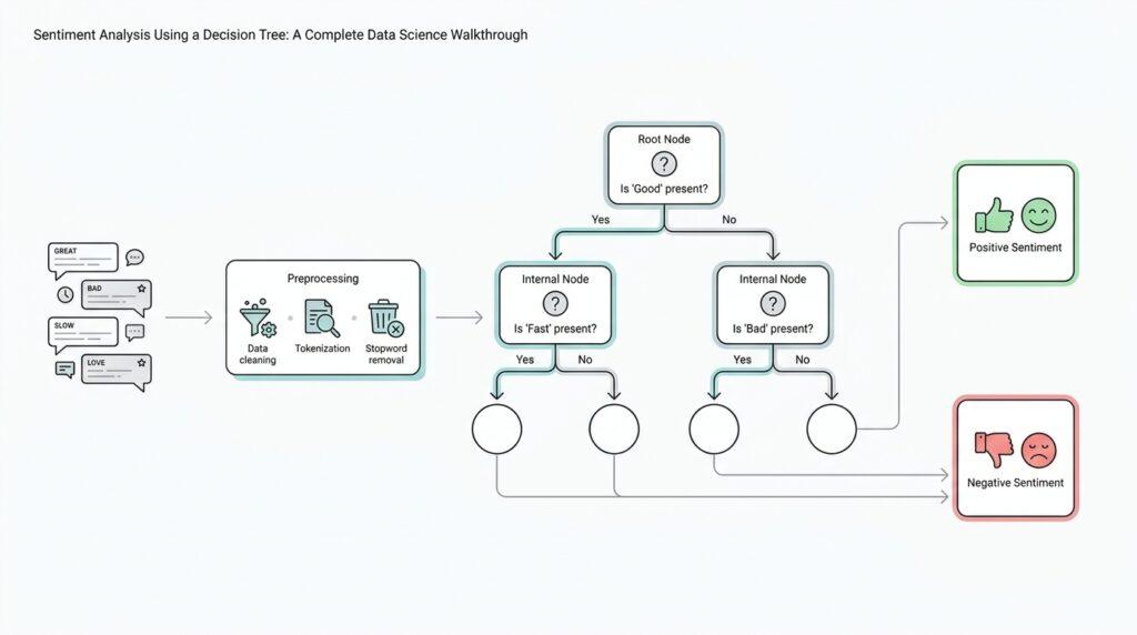
Word handling is the next place where beginners often pause, because this is where text cleaning starts to feel more like translation than tidying. A token is a single piece of text, usually a word, and tokenization means splitting a sentence into those pieces. Once the review is broken into tokens, we can remove common stopwords, which are words like “the,” “is,” and “and” that usually carry little signal on their own. That said, sentiment analysis has one important twist: words like “not” and “no” may look small, but they can flip meaning completely, so we should treat them with care instead of deleting them automatically.
Here is a simple example of what this kind of cleaning might look like in code:
import re

def clean_text(text):
    text = text.lower()
    text = re.sub(r'<.*?>', '', text)
    text = re.sub(r'[^a-z\s]', '', text)
    text = re.sub(r'\s+', ' ', text).strip()
    return text

df['clean_review'] = df['review'].apply(clean_text)
This function does a few quiet but important jobs. It lowers the text, removes HTML tags, drops punctuation and numbers, and trims extra spaces. After that, the dataset has a cleaner clean_review column that is easier to transform into features for the decision tree. That new column does not magically solve sentiment analysis, but it gives us a much more stable starting point.
Another useful step is to think about word form, because people often express the same idea in slightly different ways. The words “liked,” “likes,” and “liking” all point to the same root idea, and methods like stemming and lemmatization help bring them together. Stemming cuts words down to a rough base form, while lemmatization turns them into a dictionary form with a bit more linguistic care. In beginner-friendly projects, this can reduce noise and help the decision tree see repeated patterns more clearly, though it is worth remembering that over-normalizing text can sometimes erase useful nuance.
As we clean text data, we are really making a series of small judgment calls. We decide what counts as noise, what counts as meaning, and what the model should be allowed to notice. That is why good cleaning is part technical skill and part careful listening: we want to preserve the emotional signal while removing the clutter around it. When we get that balance right, the sentiment analysis pipeline becomes much easier to trust.
By the time we finish this stage, the dataset feels less like a pile of comments and more like material that can be measured, compared, and learned from. The cleaned text is now ready for the next transformation, where we will turn words into numbers so the decision tree can begin its work.
Converting Text to Features
Now that the reviews are clean, we meet the next practical roadblock: a decision tree cannot stare at a sentence and understand it the way you do. It needs numeric features, which are measurable pieces of information the model can compare and split on. So in sentiment analysis, we turn each review into numbers, and that process is often called feature extraction or text vectorization. If you have been wondering, “How do we convert text to features for a decision tree?”, this is the moment where the answer starts to take shape.
The easiest way to picture this is to think of each review as a shopping list. A model does not care whether the list sounds enthusiastic or annoyed; it wants to know which words appear and how often they show up. That is why one common approach is the bag of words method, which treats a text as a collection of words and counts them without paying attention to word order. We lose some sentence structure, but we gain something the decision tree can actually work with: a table of numbers.
In practice, this table is built by a vectorizer, which is a tool that turns text into a numeric representation. Each column usually stands for one word in the vocabulary, which is the full set of unique words the model sees during training. Each row stands for one review, and each cell shows how strongly that word appears in that review. The result feels a little like a crossword grid where every word has its own seat, and every review fills those seats with counts or weights.
Here is what that looks like in code:
from sklearn.feature_extraction.text import CountVectorizer

vectorizer = CountVectorizer()
X = vectorizer.fit_transform(df['clean_review'])
This small block creates a bag-of-words representation of the cleaned text. The fit_transform step teaches the vectorizer which words belong in the vocabulary and then converts each review into a row of counts. What you get back is usually a sparse matrix, which means most of the values are zero because any single review uses only a tiny fraction of all possible words. That sparse format keeps memory use manageable, which matters once your dataset grows beyond a handful of rows.
Sometimes raw word counts are enough, but sentiment analysis often benefits from a smarter weighting scheme called TF-IDF, short for term frequency-inverse document frequency. Term frequency means how often a word appears in one review, while inverse document frequency means how rare that word is across all reviews. The idea is simple: common words that appear everywhere should matter less, while words that show up in more distinctive reviews should matter more. In plain language, TF-IDF helps the model hear the useful words over the background chatter.
That distinction matters because not every repeated word tells the same story. A word like “movie” may appear in almost every review and say very little about whether the feeling is positive or negative. A word like “excellent,” “boring,” or “disappointing” usually carries much more sentiment signal, so TF-IDF gives it more weight. For a decision tree, those weighted numbers can create clearer splits, which is often exactly what we want when we are trying to separate positive reviews from negative ones.
Here is a simple TF-IDF version:
from sklearn.feature_extraction.text import TfidfVectorizer

vectorizer = TfidfVectorizer()
X = vectorizer.fit_transform(df['clean_review'])
At this point, the text has become a matrix of features that the decision tree can read like a structured table. Each review now lives as a row of numbers, and each number captures something about the language inside it. That transformation is the bridge between human expression and machine learning, and it is the reason the rest of the sentiment analysis workflow can move forward with confidence. Once the words are in numeric form, we are ready to hand them to the model and let it start learning which patterns tend to sound happy, angry, or somewhere in between.
Splitting Train and Test
Now that the reviews have been cleaned and turned into numbers, we reach a quiet but important crossroads: how do we split train and test data for sentiment analysis? This is the moment where we decide which examples the decision tree will study and which examples we will hide away for later. It may feel a little like giving a student a practice exam and then saving a surprise quiz for the end, but that surprise is what tells us whether the model actually learned or only memorized.
The training set is the portion of data the model sees during learning, and the test set is the portion we keep untouched until the end. In decision tree sentiment analysis, this separation matters because the tree can become very confident very quickly, especially when it sees the same patterns again and again. If we let it learn from everything and then judge it on the same examples, we do not really measure skill; we measure recall. A proper train and test split gives us a fairer view of how the model might behave on new reviews it has never seen before.
We usually make that split after feature extraction, when the text has already become a matrix of numbers and the labels are ready alongside it. At this stage, we want the input features in one place, often called X, and the target labels in another place, often called y. The target is the answer we want the model to predict, such as positive or negative sentiment. By separating features from labels first, we make the split cleaner and keep the workflow easy to follow.
Here is the kind of code that usually does the job:
from sklearn.model_selection import train_test_split

X_train, X_test, y_train, y_test = train_test_split(
    X, y, test_size=0.2, random_state=42, stratify=y
)
This small block creates the train/test split in a way that feels simple on the surface but carries a lot of meaning underneath. test_size=0.2 means 20% of the data goes into the test set, while 80% becomes training data. random_state=42 sets a fixed random seed, which is a starting point for randomness that helps us reproduce the same split later. stratify=y keeps the class balance similar in both sets, which is especially useful when positive and negative reviews are not evenly distributed.
That last part is worth lingering on because it solves a problem beginners often miss. If we split sentiment data without care, we might end up with a test set that contains far more positive examples than negative ones, or the reverse. Then our decision tree could look better or worse than it really is simply because the test set was lopsided. Stratified splitting acts like a careful host who makes sure both groups get a fair seat at the table.
We also want to keep the test set completely separate from the training process. That means we do not use it to choose features, tune the decision tree, or make cleanup decisions after the fact. This is called avoiding data leakage, which happens when information from the test set accidentally slips into training and gives the model an unfair advantage. Data leakage can make a model look polished during development and disappointing in real use, so keeping the train and test split clean is one of the most important habits we can build.
Once the split is done, the story becomes more concrete. The decision tree learns from X_train and y_train, and later we ask it to predict labels for X_test. That delayed check is where we start to see whether the model understands sentiment patterns in a meaningful way. If it performs well there, we have a stronger reason to trust the next steps, because the model is not only repeating what it has already seen. It is handling new text, which is exactly the skill we need in sentiment analysis.
So this stage is not just a technical formality. It is the point where we turn a pile of labeled reviews into a true learning experiment, with one half for practice and one half for proof. When we split train and test carefully, we give the decision tree a fair chance to learn and ourselves a fair chance to judge what it has learned.
Training the Decision Tree
Now that the reviews have been turned into numbers and split into training and test sets, we finally reach the part where the decision tree starts learning from the sentiment analysis data. This is the moment where the model begins to act like a very patient question-asker, looking at one feature after another and deciding how to separate positive reviews from negative ones. If you have ever wondered, “How does a decision tree learn sentiment from text features?”, this is the stage where the answer becomes visible.
Training means we show the model the examples in X_train and the correct answers in y_train, then let it discover patterns on its own. The tree does not memorize entire reviews word for word; instead, it searches for splits that group similar labels together. Think of it like sorting a stack of postcards into two piles by asking, “Does this review contain a word that usually appears in positive text?” Each split narrows the pile, and each new branch makes the separation a little more focused.
Under the hood, the tree needs a way to judge whether a split is useful, and that is where impurity comes in. Impurity means how mixed the labels are inside one group, so a node with only positive reviews is pure, while a node with both positive and negative reviews is mixed. A training algorithm often uses Gini impurity or entropy, which are two common ways to measure that mix. Lower impurity means the tree has done a better job of separating the classes, so the model keeps choosing splits that reduce confusion as much as possible.
Here is what that looks like in code:
from sklearn.tree import DecisionTreeClassifier

model = DecisionTreeClassifier(random_state=42)
model.fit(X_train, y_train)
This small block is where the real training happens. The DecisionTreeClassifier is the model type, and fit means “learn from these examples.” After this line runs, the tree has built its branches based on the training data, and it has formed a set of rules that connect word patterns to sentiment labels. In a sentiment analysis workflow, this is the point where raw text features turn into an actual predictive model.
Of course, a trained tree can become too eager if we let it grow without limits. A very deep tree may keep splitting until it learns tiny quirks in the training set, including accidental noise that will not help on new reviews. That problem is called overfitting, which means the model performs very well on familiar data but struggles when it sees fresh examples. To keep the tree from becoming too complicated, we often set limits such as max_depth, which controls how many levels the tree can grow.
For example, a smaller tree may look less impressive at first, but it often gives better results in practice because it learns the broad patterns rather than the memorized details. You might also see settings like min_samples_split or min_samples_leaf, which tell the tree to wait until it has enough examples before making a new branch or ending in a leaf. A leaf is the final stopping point in the tree, where the model makes its prediction. These settings work like guardrails, keeping the decision tree from rushing into overly specific rules.
Training also gives us a chance to think about balance, because a tree learns best when both sentiment classes are represented fairly in the training data. If one class appears much more often, the tree may lean toward that class unless the patterns are especially strong in the minority side. That is why the earlier train-test split mattered so much: we wanted the model to learn from a realistic mix of examples, not from a skewed pile that would distort its sense of the data. Good sentiment analysis depends on that balance as much as it depends on the words themselves.
Once the tree is fit, it becomes ready for the next step: making predictions on text it has never seen before. At that point, we will be able to ask whether the model learned useful sentiment patterns or merely followed the training data too closely. For now, though, the important thing is that training has turned our cleaned, vectorized reviews into a structured set of branching rules, and that structure is what lets the decision tree begin doing its job.
Measuring Model Performance
Once the decision tree has learned from the training data, the next question is the honest one: how well does it handle reviews it has never seen? Measuring model performance in sentiment analysis starts with the test set, because that is where we check whether the tree is recognizing positive and negative language rather than memorizing patterns. Accuracy tells us the fraction of correct predictions, while precision, recall, and F1 score each show a different angle of the result. If you are asking, “How do I measure model performance for sentiment analysis in a way that feels fair?”, this is the toolkit we reach for first.
That is why we do not stop at accuracy. In sentiment analysis, a model can get many labels right and still make the wrong kind of mistake in a way that matters, so we ask precision and recall to separate those errors. Precision asks how often the model is correct when it predicts a positive sentiment, and recall asks how many of the truly positive reviews it manages to catch. F1 score then combines precision and recall as a harmonic mean, which keeps one strong number from hiding a weakness in the other.
A confusion matrix gives us the clearest picture of those mistakes. It lays out true negatives, false positives, false negatives, and true positives so we can see exactly where the decision tree slips. In a sentiment analysis model, that means we can tell whether the tree is confusing positive reviews with negative ones, or whether it is leaning too cautiously in one direction. The matrix turns a single score into a small map of model behavior, and that map is often more useful than a lone percentage.
Here is a compact way to read those numbers after prediction:
from sklearn.metrics import accuracy_score, precision_score, recall_score, f1_score, confusion_matrix, classification_report

y_pred = model.predict(X_test)

print('Accuracy:', accuracy_score(y_test, y_pred))
print('Precision:', precision_score(y_test, y_pred))
print('Recall:', recall_score(y_test, y_pred))
print('F1:', f1_score(y_test, y_pred))
print(confusion_matrix(y_test, y_pred))
print(classification_report(y_test, y_pred))
The classification_report gives a short summary of the main classification metrics, which makes it a handy companion to the confusion matrix when we want a quick read on the sentiment analysis model. It is the kind of output you can scan once, then return to with more confidence when the numbers start telling a story.
If the test score looks good, we still want a second opinion. Cross-validation splits the data into multiple folds, trains several times, and averages the scores so one lucky split does not fool us. In scikit-learn, cross_val_score uses 5-fold cross-validation by default when cv=None, and classifiers with binary or multiclass labels use StratifiedKFold so each fold keeps the class mix balanced. That makes the performance estimate steadier and gives us a better sense of how the decision tree may behave on new text.
By the time we look at accuracy, precision, recall, F1, the confusion matrix, and cross-validation together, the model performance story becomes much clearer. We stop guessing whether the sentiment analysis model is good and start seeing where it is strong, where it is shaky, and what kind of mistakes it prefers to make. That fuller view is what prepares us for the next step, because once we understand the numbers, we can begin tuning the tree with purpose instead of hope.