Big Six Overview
Every time you touch a database in production you’re relying on a small set of commands to keep data correct, performant, and auditable; mastering these SQL commands is non-negotiable for every developer. In the first 100 lines of a migration or the last query in a performance incident, the difference between a controlled change and a critical outage is how you use SELECT, INSERT, UPDATE, DELETE, CREATE, and ALTER. How do you decide which command to use when a feature request touches both schema and live data? We’ll frame that decision-making so you can act with confidence.
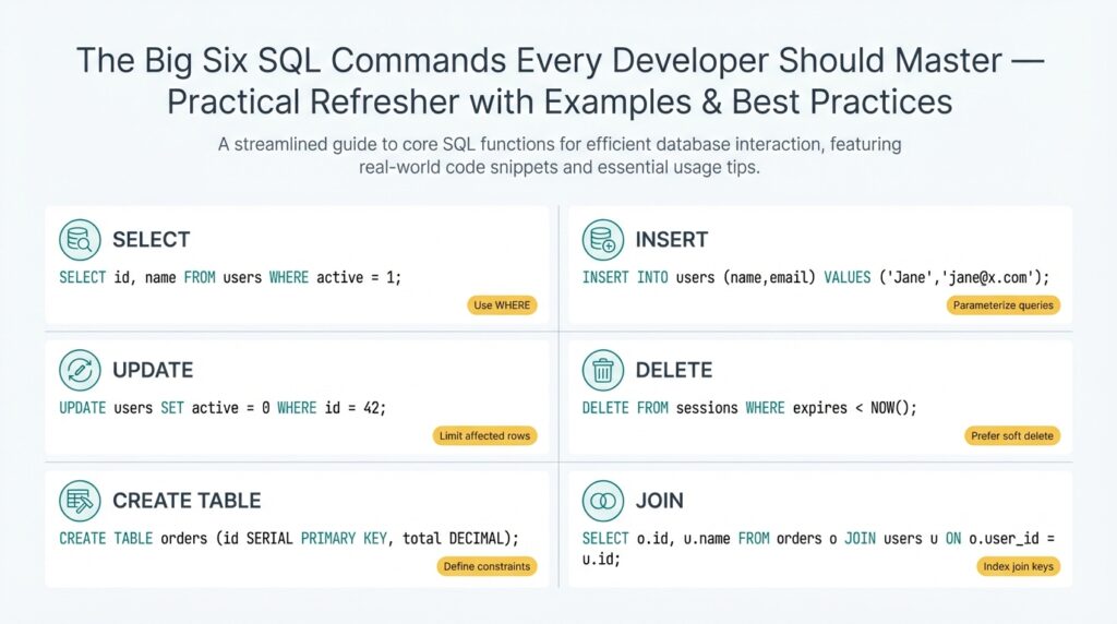
Start with an operational definition for each command so you and your team share vocabulary. SELECT retrieves rows and drives read-heavy features like dashboards and analytics; INSERT adds new rows for events, user actions, and backlog items; UPDATE mutates existing rows to reflect state changes; DELETE removes rows when data retention or business rules require it; CREATE defines new tables, indexes, or other schema objects; ALTER changes schema without full rebuilds. Using these terms precisely helps during code reviews and incident postmortems.
These six commands fall into two practical categories: DML (Data Manipulation Language) and DDL (Data Definition Language). DML—SELECT, INSERT, UPDATE, DELETE—handles the day-to-day read/write traffic your application generates, so you optimize it for concurrency, transactions, and idempotency. DDL—CREATE and ALTER—changes the database structure and therefore requires migration planning, schema-version control, and rollback strategies. Because DDL can lock metadata and cause service interruptions, coordinate ALTER operations with maintenance windows or online-migration tools.
When we apply these commands in real systems we follow patterns that reduce risk. Always use transactions around multi-step changes (BEGIN; UPDATE …; INSERT …; COMMIT;) to maintain atomicity and leverage explicit locking only when necessary to avoid deadlocks. Prefer parameterized queries to prevent SQL injection and make query plans cacheable. For updates and deletes on large tables, prefer batched operations with a cursor or LIMIT/OFFSET loop to avoid long-running locks and to keep replication lag bounded. These practices make SELECTs more reliable and INSERT/UPDATE/DELETE operations predictable under load.
Practical examples clarify trade-offs you’ll face. If you need to add a new nullable column and backfill values for millions of rows, use CREATE to add the column, then perform batched UPDATEs while monitoring replication lag; avoid an instant ALTER that rewrites the table unless you’re using an online DDL tool. For app-level migrations where data must be transformed, INSERT into a new table built with CREATE, verify integrity with SELECT queries, then swap pointers or rename tables with ALTER to minimize downtime. These patterns reduce risk compared to in-place destructive changes and preserve a clear rollback path.
Building on this foundation, the next sections will walk through concrete examples, SQL snippets, and checklist-driven best practices for each command so you can implement them safely. We’ll show real-world queries you can adapt, demonstrate how to measure impact with EXPLAIN and monitoring, and explain when to prefer schema-first versus data-first approaches. By internalizing the trade-offs between SELECT/INSERT/UPDATE/DELETE and CREATE/ALTER, you’ll make faster, safer changes and reduce blast radius during deployments.
SELECT: Choosing Columns & Expressions
Building on this foundation, the single most impactful decision you make when reading data is what you project in the SELECT list—because the fields you request drive I/O, CPU, network transfer, and downstream complexity. How do you decide which columns to select to balance performance and readability? Start by treating the projection as an explicit contract between your application and the database: list only the attributes your code needs, name computed values clearly, and avoid surprises that force refactors later.
Prefer explicit column lists over SELECT * for stability and performance. An explicit list makes intent obvious in code reviews, prevents accidental data leaks when schema changes, and keeps row widths small which reduces disk and network I/O. For example, prefer:
SELECT id, user_id, total_cents, created_at
FROM orders
WHERE created_at >= DATE_TRUNC('month', CURRENT_DATE);
instead of:
SELECT * FROM orders WHERE created_at >= DATE_TRUNC('month', CURRENT_DATE);
Explicit columns also make query plans easier to reason about in EXPLAIN output and avoid needless client-side parsing of unused fields.
Use expressions in the projection when you need derived values, but be intentional about their cost. Expressions are any computation in the SELECT list—arithmetic, function calls, CASE statements, JSON extraction, or aggregates. These are great for concise result sets (for example computing a status, rounding money, or formatting timestamps), but each expression consumes CPU across every qualifying row. If you write:
SELECT id, amount_cents / 100.0 AS amount,
       CASE WHEN amount_cents > 10000 THEN 'high' ELSE 'normal' END AS risk_bucket
FROM transactions;
you get useful, application-ready values, but if transactions is huge and this query runs frequently, consider persisting the risk_bucket or precomputing amounts in ETL to avoid repeated CPU work.
Be deliberate with complex expressions that touch JSON, regex, or user-defined functions because they can bypass index benefits implicitly and amplify latency. JSON->path operations, regex_search, or heavy string manipulation are fine for ad-hoc reporting, but for production read paths prefer indexed generated columns or use LATERAL/CROSS APPLY to isolate expensive logic and limit rows first. For example, extract only necessary JSON keys and project them as typed columns in a materialized view or persisted computed column so your OLTP query remains shallow.
Decide whether to compute in SQL or in the application by measuring the trade-offs between network transfer and server CPU. If multiple consumers need the same derived column, centralize the logic in the database (view, function, or materialized view) to reduce duplication and inconsistencies. Conversely, when a transform is heavy and infrequently used, push it into a background job or service that writes a ready-to-read column; this keeps hot read paths fast and predictable. Window functions provide powerful per-row context in the projection, but they often force sorting and additional memory—use them judiciously and test with representative data sizes.
Finally, make observability and maintainability part of the projection decision. Name computed columns clearly, document non-obvious expressions near the query, and add comments when you rely on persisted expressions or materialized views. Measure the impact of projection choices with EXPLAIN/ANALYZE and latency-sensitive production traces; if a SELECT suddenly becomes the bottleneck, the first thing to check is what you’re projecting. Taking these steps lets us keep read queries compact, predictable, and efficient while giving applications the exact shape of data they need to operate.
FROM: Tables, Views, Sources
Building on this foundation, the single biggest decision you make when assembling a SELECT is which objects you read from and why. The FROM clause defines the data sources—base tables, views, derived tables, CTEs, or set-returning functions—and that choice drives I/O, locking behavior, and the optimizer’s ability to push down filters. If you treat the FROM clause as an explicit contract between the query and the storage layer, you avoid surprises in performance and semantics downstream.
Start by differentiating the common source types you’ll encounter in production: persistent tables hold the canonical state; views encapsulate projection or joins; materialized views persist precomputed results for read-heavy workloads; derived tables (subqueries) and CTEs provide scoped transforms; and external sources (foreign tables, files, or table-valued functions) bring data from outside your primary storage. Each source has different cost characteristics—tables are I/O-bound but indexable, views are logical (and may hide complexity), while materialized views trade storage for faster reads. Choose the simplest source that expresses intent and keeps read paths predictable.
Views are powerful for reuse and security, but they also conceal execution details that matter for performance. When should you select from a view versus the underlying table? Use views when you need a consistent projection, access control, or to centralize complex joins used by many consumers. Prefer querying underlying tables when you must tune indexes, push predicates, or JOIN differently for a particular query. If a view is slow and frequently read, consider converting it to a materialized view or maintaining a summarized table that you refresh on a schedule or via incremental ETL.
Make the optimizer’s job easier by projecting and filtering as early as possible in the FROM clause. Alias every source clearly and include schema qualifiers to avoid ambiguity and accidental cross-schema scans. Push selective WHERE predicates before expensive joins and prefer indexed join keys; for example:
SELECT o.id, o.total_cents, c.region
FROM public.orders o
JOIN public.customers c ON o.customer_id = c.id
WHERE o.created_at >= '2026-01-01' AND c.active = true;
Applying the date filter to orders first reduces rows before the join, which usually shrinks memory and sort footprints.
Derived tables, CTEs, and LATERAL joins let you express complex logic inline, but they can change optimization behavior between engines. Some databases materialize CTEs (creating a temporary snapshot) which can be helpful for correctness or harmful for performance; others inline them into the main plan. For heavy transforms, test both a CTE and an equivalent subquery or temporary table and compare EXPLAIN ANALYZE results. When you need reusable intermediate results across multiple queries, persist them instead of recalculating in many SELECTs.
In large-scale systems you must think beyond the single query: partitioning, statistics, and appropriate indexes determine how efficient reads from big tables are. Design join keys that align with partitioning and avoid scanning the full table for common access patterns by adding covering indexes or using partition pruning. For backfills or analytics that read massive tables, prefer batch processing, parallel scans, or materialized aggregates to keep OLTP latency predictable while you operate on archival data.
Practical observability completes the pattern: always validate source choices with EXPLAIN/ANALYZE and production traces, and add comments to views that encapsulate non-obvious joins or filters. When you change a view or swap a materialized table into production, run representative queries to confirm plans and watch replication lag or query latency for regressions. In the next section we’ll take these source-selection principles and show how they affect joins, projections, and index usage in concrete examples so you can optimize read paths confidently.
WHERE: Filtering Rows Effectively
Most performance bugs start in the WHERE clause: a predicate that forces a full table scan, applies a function to every row, or accidentally widens the working set. When you’re filtering rows, think in terms of selectivity and index usage first—those two factors determine whether a query runs in milliseconds or minutes. Front-load predicates that match your indexes and avoid transformations on indexed columns so the database can perform predicate pushdown and use the index efficiently. How do you avoid full table scans and keep reads predictable under load?
A predicate is any Boolean expression that narrows the result set, and whether a predicate is sargable determines if an index can help. Define sargable on first use: a predicate is sargable when the optimizer can use an index to limit row access rather than evaluating the expression on every row. Comparisons like =, >, >=, BETWEEN, and IN against raw columns are sargable; wrapping a column in a function (for example, DATE(created_at) = ‘2026-03-01’) usually breaks sargability. When you write filters, prefer expressions that leave the column alone and move transformations to constants or computed columns.
Practical rewrites make a huge difference. For example, replace
WHERE DATE(created_at) = '2026-03-01'
with
WHERE created_at >= '2026-03-01' AND created_at < '2026-03-02'
This preserves an index on created_at and enables index range scans instead of a sequential scan. Similarly, prefer column = value over LIKE ‘%value%’ when you expect indexable matches; if you need substring search, consider full-text indexes or trigram indexes that are designed for that workload.
Composite and covering indexes change how you design predicates. When an index has multiple columns, the leftmost prefix matters: put the most selective, frequently-queried column first and then include additional columns needed to cover queries so the database can satisfy the SELECT from the index alone. That reduces I/O and avoids lookups to the base table. Remember that the optimizer decides execution order, so order predicates by selectivity in your mental model, but align schema and indexes to the access patterns you measure.
Nulls and three-valued logic are another common source of surprises when filtering rows. IS NULL and IS NOT NULL are not equivalent to = NULL or != NULL, so be explicit. If a frequent filter is is_active = true, you can create a partial index (WHERE is_active = true) to speed up reads and reduce index size; partial indexes are powerful when a small subset of rows answers most queries. Use partial or filtered indexes to support common filters and keep index maintenance affordable.
Choosing between EXISTS, IN, and JOIN affects performance when your WHERE depends on another table. EXISTS with a correlated subquery often short-circuits as soon as a matching row is found, which makes it efficient for existence checks. IN can be fine for a small, bounded list, but for large sets prefer a JOIN or a hashed temporary set; for anti-joins, prefer NOT EXISTS over NOT IN when NULLs are possible. Test each pattern with EXPLAIN ANALYZE on representative data to see which plan the optimizer produces.
For large-scale updates, deletes, or backfills, use WHERE to drive batching and keep locks short: delete 10k rows per transaction, commit, and repeat while monitoring replication lag. When filtering rows in OLTP paths, prefer indexes and covering projections so you avoid touching the heap. Add pragmatic guards in production code—deadman limits, dry-run flags, and explicit ORDER BY with LIMIT for destructive operations—to prevent accidental full-table changes.
Measure and iterate: run EXPLAIN/ANALYZE, inspect filter estimates versus actual rows, and check whether predicates are being pushed down into index scans or executed post-join. Observability clarifies whether your WHERE predicates, indexes, or data distribution are the real bottleneck. Taking this approach keeps filtering rows predictable and prepares us to tune join strategies and index designs in the next section.
GROUP BY & HAVING: Aggregation Rules
Grouping and aggregation turn row-level data into the summaries your dashboards and reports rely on, so understanding GROUP BY and HAVING rules saves you from subtle bugs and incorrect results. The fundamental contract is simple: every expression in the SELECT list must either be an aggregate (sum, count, avg, min, max) or appear in the GROUP BY clause; otherwise different SQL engines will raise an error or return nondeterministic rows. Building on our earlier discussion of projection and filtering, treat grouping as a projection-level constraint that reshapes the result set before ORDER BY or LIMIT apply. When you design summaries, decide first which dimensions you need to group by and which values you need to aggregate, because that choice drives index design and query shape.
The core semantic rule prevents ambiguity: if you include a non-aggregated column that isn’t grouped, the database cannot deterministically pick one value from the multiple rows in that group. This rule exists because aggregation collapses many rows into one row per group, and the SELECT list must describe that single row unambiguously. In practice, some engines tolerate nonstandard extensions that pick a “first” value, but relying on that makes queries nonportable and brittle. For robust code reviews and predictable plans, require that all non-aggregates are explicit grouping keys and keep expressions simple enough that the optimizer can reason about them.
Concrete examples make the rule actionable. Suppose you want total spend per customer from an orders table: run this query to compute totals correctly:
SELECT customer_id, SUM(total_cents) AS total_cents
FROM orders
WHERE created_at >= '2026-01-01'
GROUP BY customer_id;
Contrast that with the common mistake of selecting created_at without grouping; the database will either error or return an arbitrary timestamp for each customer. If you need the earliest order timestamp per customer, express it as an aggregate explicitly (MIN(created_at)) so the intent and plan are clear.
Filtering rows versus filtering groups is another place to apply rules carefully: WHERE filters input rows before aggregation, while HAVING filters the aggregated groups after the summary is produced. When should you use HAVING instead of WHERE? Use HAVING when the predicate depends on an aggregate value, for example to only keep customers with more than five orders:
SELECT customer_id, COUNT(*) AS orders
FROM orders
GROUP BY customer_id
HAVING COUNT(*) > 5;
If you try to put COUNT(*) > 5 in WHERE the optimizer will reject it because the count doesn’t exist yet at that stage of execution.
Take grouping further with advanced constructs when you need multiple rollups in a single pass: GROUPING SETS, ROLLUP, and CUBE let you produce hierarchical or cross-dimensional aggregates without repeating queries. These constructs are powerful for multidimensional reporting but increase plan complexity and memory usage because the engine must produce multiple aggregate rows per input row. Also remember the relationship between aggregation and window functions: window functions compute values across partitions of already-selected rows and are applied after aggregates when used together, so choose between per-group aggregates and per-row windowed metrics depending on whether you want a collapsed summary or contextual values per row.
Performance and maintainability matter as much as correctness when you aggregate at scale. Favor grouping on low-cardinality, highly selective dimensions and avoid grouping on high-cardinality text or UUID columns unless you truly need that granularity. Where recurring reports are heavy, pre-aggregate into materialized views or maintain incremental summary tables to shift work off critical OLTP paths. Always validate plans with EXPLAIN ANALYZE, watch memory and temp-file usage for sort-heavy aggregates, and consider partial or filtered aggregates when only a subset of groups matters. Next we’ll apply these aggregation rules to multi-table queries and show how join order and indexes change both correctness and performance.
ORDER BY: Sorting and Performance
Sorting is one of the biggest implicit costs you pay when producing ordered result sets, and it shows up as CPU, memory, and temporary-disk usage before your application ever sees a row. If you ask the database to return rows in a particular order, the engine either performs an index-ordered scan or runs a sort operation over the working set; understanding which path it chooses is the key to predictable performance. How do you decide whether to rely on an index-ordered scan or let the engine sort in memory or on disk? We’ll walk through the trade-offs and actionable patterns you can apply in production.
Start by treating index ordering as a free sort when possible: if your query’s ORDER clause matches an index key (including direction), the optimizer can produce rows in order without an explicit sort step. Create composite indexes that mirror your most common ORDER and WHERE combinations so the engine can perform an index-only scan or a covering index scan and avoid copying rows into a sort buffer. For example, when you frequently request the latest activity per user, an index on (user_id, created_at DESC) lets you run:
SELECT id, user_id, payload, created_at
FROM events
WHERE user_id = ?
ORDER BY created_at DESC
LIMIT 10;
and return the top-N directly from the index with minimal I/O.
When an index can’t satisfy ordering, the database runs a sort operation that uses memory (a sort buffer) and spills to temporary files on disk if the working set exceeds that memory. Sorting large joined results or wide projections amplifies both CPU and I/O cost, so push selective WHERE predicates and projections early—filter rows before the join and select only the columns you need—to shrink the set that must be sorted. Taking this concept further, if you’re producing paginated reads, prefer keyset pagination (also known as cursor or seek pagination) over OFFSET/LIMIT, because OFFSET forces the engine to sort and skip N rows before returning the page, which becomes increasingly expensive as N grows.
In multi-table queries the sort point matters: for example, if you join several tables and then ORDER, the optimizer may need to materialize or buffer the join result before sorting. We’ve covered pushing filters and choosing join keys earlier; now emphasize ordering-aware join and index design. If your ORDER depends on a column from the driving table, push the predicate to reduce rows first; if it depends on a joined column, consider denormalizing or maintaining a pre-sorted summary column to avoid costly post-join sorts. Partial indexes or materialized views that maintain pre-ordered subsets can shift sort work offline and improve runtime performance.
Collation, NULL placement, and sort direction are small semantic details that affect whether an index is usable for ordering. Different collations change the byte-level order of strings, and some databases don’t allow a single index to serve both ASC and DESC efficiently for multi-column keys unless you explicitly define directions when creating the index. If your application mixes case-insensitive comparisons or locale-aware orderings with ordering requirements, test whether the index is truly being used by inspecting EXPLAIN plans; otherwise you’ll get a hidden sort that negates the index benefits.
Measure and iterate: always confirm assumptions with EXPLAIN ANALYZE and representative data volumes. Look for an explicit SORT node, check sort memory and temp-file usage, and validate whether a top-N optimization (LIMIT with ORDER) is applied. When you identify expensive sorts, try one of three patterns: create an index that matches ORDER+WHERE, switch to keyset pagination, or precompute ordered results into a materialized view or summary table. Taking these steps lets us manage sorting costs predictably and keep query latency bounded as data grows, which prepares us to discuss how ordering interacts with aggregates and window functions in the next section.