Audit Storage-Heavy Tables
After the schema work, the next surprise is often where the bytes actually live. In Cloud Spanner, a table can look harmless until its base rows, indexes, and even change-stream tables quietly become the most expensive part of the database. A good audit starts with the total database storage metric and Spanner’s built-in table-size history, because those give you the clearest first look at which objects are carrying the weight.
The first question to ask is: which objects are largest right now, and which ones keep growing? SPANNER_SYS.TABLE_SIZES_STATS_1HOUR lists table and index sizes in bytes, includes data versions, and gives you a historical view instead of a single snapshot. That makes it useful for spotting storage-heavy tables that are steadily climbing, not just temporarily noisy. A query for the largest objects in the most recent interval often surfaces the obvious suspects quickly.
Then we pair size with activity. SPANNER_SYS.TABLE_OPERATIONS_STATS_* tracks reads, writes, and deletes for tables and indexes, so you can tell whether a large table is hot or just sitting there like a packed closet nobody opens. This matters because one write to a table also increments the count for its indexes, which helps you see when index maintenance may be amplifying storage pressure. If size is rising faster than traffic, you may be looking at old data, redundant indexes, or a column that no longer earns its keep.
Indexes deserve a careful look because Spanner stores index data like tables under the hood. Non-interleaved indexes live in root tables and often sit away from the base data, which adds extra work on writes and extra splits to consult on reads; STORING copies columns into the index, and NULL_FILTERED helps keep sparse indexes from copying more than they need. That tradeoff can be useful, but it also means every extra convenience column has a storage price. When a table feels too big, the real culprit is often an index that mirrors too much of it.
Large columns deserve the same honesty. Spanner’s design guidance says to consider placing large columns in non-interleaved tables when they are accessed less often, while keeping related data together so the rows you read and write together stay nearby. Think of it like moving bulky holiday gear out of the hallway and into a storage room: the everyday path gets lighter, and the rarely used items still have a home. This is where Cloud Spanner schema design becomes practical, because the goal is not fewer bytes at any cost, but fewer expensive bytes in the wrong place.
As you audit, keep one last detail in mind: storage drops do not always appear immediately. Spanner compacts deleted data in the background, so the storage-utilization metric can lag after cleanup, especially after large deletions. That means the best read on storage-heavy tables comes from combining size trends, operation counts, and a look at whether a table is still worth its footprint. Once we know which objects are both large and active, we can decide whether to trim them, split them apart, or retire the access path entirely.
Choose Compact Primary Keys
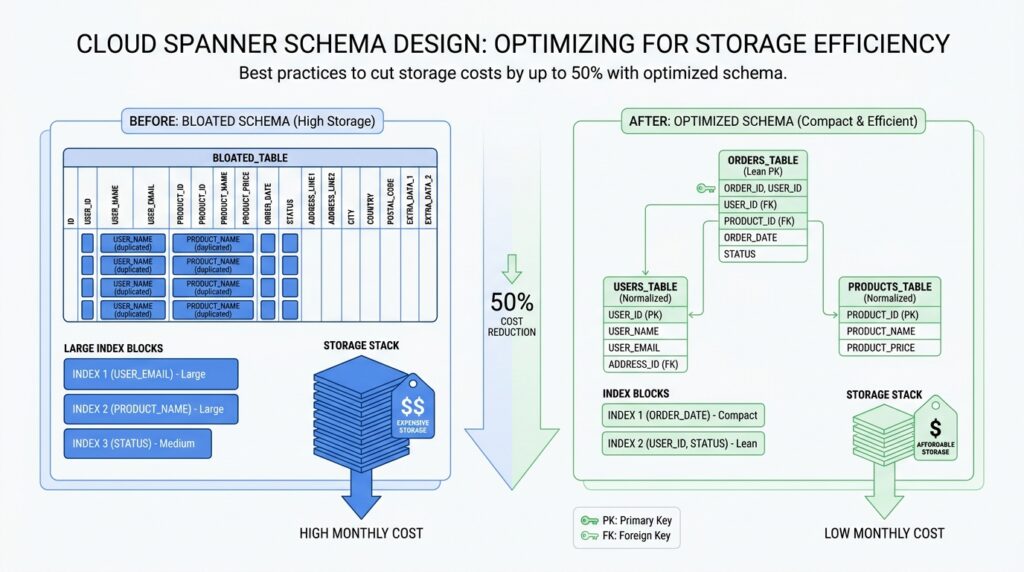
After you trim the biggest tables, the next place to look is the label on each row itself. In Cloud Spanner, the primary key is not only how a row is found; it also determines row order, and Spanner automatically indexes primary key columns for quick lookup. That means a long or bulky key does more than describe a record — it becomes part of the database’s physical shape. Choosing compact primary keys keeps that shape lighter, which is one of the quietest ways to reduce Cloud Spanner storage costs.
What makes a primary key “compact” in Cloud Spanner schema design? Think of it like the shipping label on a package: it should identify the box without becoming the box. Spanner stores rows in lexicographic order by PRIMARY KEY, so each extra key column or wide key value becomes part of the sorted path the database maintains. Spanner also limits the size of a primary key or index key to 8 KiB per row, which is generous, but not a reason to spend bytes casually. Short, stable keys keep the row layout easier to manage and leave more room for actual data.
The easiest trap is using a key that is too descriptive. A primary key that embeds meaning, timestamps, or long text can feel convenient at first, but it usually grows faster than the row itself. If you need a unique identifier, Spanner supports UUID version 4, and it can store it as STRING(36), a pair of INT64 columns, or BYTES(16). The docs also note that STRING(36) UUIDs are slightly large, so if you care about compactness, the narrower representations are worth considering.
This matters even more because the primary key does not stay alone. Spanner automatically creates an index for each table’s primary key, and secondary indexes carry all base-table key columns as part of their stored data. In plain language, every extra byte in your primary key can echo through the rest of the schema, because indexes have to carry that key around too. So when you choose a compact primary key, you are not only shrinking the base table; you are also shrinking the repeated footprint that shows up in index structures. That is why compactness pays off more than it first appears.
A good rule of thumb is to separate identity from meaning. If a row needs a customer number, order code, or human-friendly label, keep that value in a regular column instead of forcing it into the primary key unless you need it for locality or uniqueness. That is an inference from Spanner’s layout: because the key controls row order and indexing, a small surrogate key plus separate business columns usually keeps storage cleaner and gives you more freedom to change the business data later. When you do need a composite key, make each part earn its place by improving distribution or access patterns, not by carrying extra narrative.
If you are still deciding between options, a compact key is usually the one that is short, immutable, and boring in the best possible way. For many schemas, that means a numeric key, a UUID stored efficiently, or a bit-reversed sequence when you want uniqueness without hotspots. Spanner’s guidance on primary key design is really the same lesson we saw in the storage audit: avoid wasting expensive bytes on things that could live elsewhere. Once the key stays lean, the rest of Cloud Spanner schema design becomes easier to tune for both cost and performance.
Interleave Related Child Tables
After we trim the primary key, the next question is where the rows that belong together should live. In Cloud Spanner schema design, an interleaved child table is a child table that Spanner stores physically with its parent row, so related data can travel together instead of being split apart. If you want a picture, think of a parent folder with its matching papers clipped behind it rather than scattered across separate drawers. That layout matters most when one parent row usually leads you straight to a small set of child rows, because keeping those rows close can reduce storage access and network traffic.
To make that work, the child table’s primary key has to begin with the parent table’s primary key, in the same order. Spanner then treats the parent row and its descendants as a row tree, and it tries to keep that tree inside the same split when possible. A split is the unit Spanner uses to distribute contiguous row ranges across resources, so staying inside one split avoids extra coordination. In plain language, interleaving is Spanner’s way of saying, “these rows are a family, so let’s keep the family close together.”
That is why interleaving works best for true parent-child relationships, not for tables that only meet occasionally. Google’s guidance says to model a relationship with either interleaved tables or foreign keys, but not both, and foreign keys do not imply physical colocation in storage. So if your application often reads a parent row and then immediately reads a bounded set of child rows, interleaving fits the pattern well. If the child data needs to stand on its own, or it is queried from many different paths, a separate root table may be the cleaner choice in Cloud Spanner schema design.
The cleanup story is just as important as the read path. When you want parent deletes to remove child rows automatically, the interleaved children must use ON DELETE CASCADE, and Spanner applies those deletes atomically with the parent. That makes retention rules easier to reason about, especially when old parent records should take their descendants with them. The tradeoff is that large parent-child hierarchies can run into transaction-size limits, so a design that looks neat on paper still needs a reality check on how much data each subtree can hold.
There is one last detail that keeps this decision honest: interleaving is permanent. Once you declare a table as interleaved, you cannot undo that choice in place; you would need to create a new table and migrate the data. So before we commit, we should imagine the schema a year from now, not just today’s query. If the parent and child will keep moving together, interleaving is a strong fit; if not, leaving them separate gives us more flexibility while we keep tuning Cloud Spanner schema design for cost and locality.
Reduce Secondary Index Bloat
If you’ve ever added an index and then wondered why the database got bigger instead of lighter, you’re in the right place. In Cloud Spanner, secondary indexes do more than point to rows; Spanner stores the base table’s key columns in every secondary index, and it also stores any columns you add with STORING or INCLUDE. That means each new index can carry a little extra baggage, and once that pattern repeats across several indexes, storage costs start to rise in a way that feels sneaky rather than dramatic. The question to keep asking is: does this index earn its keep, or is it quietly creating index bloat?
The easiest place for bloat to creep in is a wide primary key. Spanner automatically indexes primary key columns, and each secondary index also repeats the base table key columns, so a bulky key gets echoed across more of the schema than you might expect. Spanner allows a primary key or index key up to 8 KiB per row, but that limit is a ceiling, not a target, and a long composite key can make every index row heavier. When you can keep identity separate from business meaning, you usually give yourself a cleaner, smaller layout that is easier to live with later.
From there, the next question is whether the index really needs all the extra columns you asked it to remember. STORING and INCLUDE are useful because they let Spanner answer a query from the index alone, but the tradeoff is straightforward: those copied values consume extra storage, and Spanner updates them whenever the base row changes. In other words, every convenience column is a suitcase you now have to carry on every trip. If you’re designing Cloud Spanner schema design for lower storage costs, keep the index narrow unless a real query benefits from the wider shape.
Sparse data gives us another gentle escape hatch. If most rows have NULL in the indexed columns, a NULL_FILTERED index can be considerably smaller and more efficient to maintain than a normal index because it leaves those rows out entirely. That matters when you only need to search the small slice of data that actually contains values, not the empty spaces around it. So when you’re asking, “Does this index really need every row?”, the answer is often no; filtering out nulls can cut down both storage and maintenance work at the same time.
The hidden cost of index bloat shows up again on writes. Spanner records write activity for tables and indexes, and a write to a table increments the write count on all indexes on that table; the bulk-loading guidance also notes that writes touching indexed data take longer because the index must be updated too. That is why a bloated index hurts twice: it takes space on disk, and it steals time from every insert, update, or delete that has to keep it current. If an index no longer supports a real query path, dropping it is often the cleanest way to reclaim both storage and write budget.
A good habit is to treat each secondary index like a borrowed tool, not a permanent fixture. Keep the key narrow, add stored columns only when a query truly needs them, filter out null-heavy rows when the data is sparse, and retire indexes that no longer pay for themselves. That is the heart of reducing secondary index bloat in Cloud Spanner: fewer copied bytes, fewer repeated updates, and a schema that stays lean enough to support the work you actually do.
Store Large Columns Separately
After we shrink keys and trim indexes, one bulky column can still drag every common read through extra work. How do you store large columns in Cloud Spanner without making every everyday lookup pay for data it rarely needs? Spanner’s guidance points us toward separating infrequently accessed large data from the hot row, because when related data is not read together, the biggest gains come from keeping the large piece out of the main path.
The mental model is easy to borrow from a closet: keep the clothes you wear daily at arm’s reach, and put the winter bins on a higher shelf. Spanner gives you that shelf with locality groups, which preserve data locality relationships across table columns, and column-level locality groups let specific columns be stored separately so they can be read more efficiently than columns grouped with the rest of the row. In practice, that means a wide table can stay wide in meaning without staying wide in the bytes it touches on every request.
This is where a large text field, compressed attachment, or other bulky payload starts to look different from the rest of the record. If the app only needs that value occasionally, Spanner’s design guidance says to consider storing large columns in non-interleaved tables, and its whitepaper notes that the benefit is strongest when the infrequently accessed data is also large. That is the same shape as keeping the everyday row lean and letting a separate, less-traveled place hold the heavy material until you actually ask for it.
The important part is restraint, because separation is not automatically better. If a column travels with the parent most of the time, clustering data together can help latency and throughput, while operations that span splits carry a bit more CPU cost and latency because Spanner has to coordinate across distributed pieces. So the rule of thumb is to separate the large column only when it behaves like an optional accessory, not when it is part of the outfit you wear every day.
A good check is to ask what your most common screens or queries actually show. If the list view, dashboard, or report only needs the title, status, and timestamp, then the heavy photo, PDF, or long payload should not sit in the hot row unless you truly need it there; Spanner can keep it logically attached while storing it separately from the columns your frequent reads depend on. That keeps Cloud Spanner schema design leaner, lowers the bytes involved in ordinary reads, and gives the large column room to grow without dragging the rest of the table along.
Delete Stale Data With TTL
Once the table has been trimmed and the indexes are under control, the next big win in Cloud Spanner schema design is often time to live (TTL), a rule that tells Spanner when a row has outlived its usefulness and can be deleted automatically. This is the moment when storage cleanup stops being a manual chore and starts behaving like a background routine. TTL can lower storage and backup costs, reduce the rows some queries need to scan, and help with retention rules, so it is one of the most practical tools for deleting stale data in Spanner.
What makes TTL appealing is that it works quietly, not dramatically. Spanner runs it in the background at low priority, checks for eligible rows regularly, and usually deletes expired data within about 72 hours; deleted storage is typically reclaimed within about seven days after compaction catches up. That delay is worth remembering, because TTL does not hide a row the instant it becomes eligible, and it does not block an insert just because the timestamp already looks old. In other words, TTL is a cleanup sweeper, not a real-time gatekeeper.
So how do we set it up without turning the schema into a puzzle? For GoogleSQL databases, you attach a row deletion policy that compares a timestamp column with an interval, and Spanner allows only one TTL policy per table. For PostgreSQL databases, the same idea appears as a TTL INTERVAL clause, and the timestamp column must be a TIMESTAMPTZ value. A row with NULL in the TTL column will not be deleted by the policy, which makes the choice of expiration column worth thinking through carefully.
This is where Cloud Spanner schema design becomes more like storytelling than housekeeping. If the data has a simple life span, a single timestamp column is enough, but if the expiration rule depends on more than one fact, Spanner lets us build a generated column first and then attach TTL to that result. That means we can express patterns like “cancelled records expire sooner” or “use the later of two dates,” while still keeping the actual deletion policy simple. One small but important caution: generated columns used for TTL cannot reference a commit timestamp column.
The same care applies when old rows have children. If a parent table uses TTL and its interleaved children should disappear with it, those children need ON DELETE CASCADE, because Spanner deletes the parent and matching descendants atomically within a batch. That works well for many family-style schemas, but very large parent-child hierarchies can run into transaction size and mutation limits, especially when indexes are involved. When that happens, Spanner recommends considering separate TTL policies on child tables, especially when a parent has a large number of children or the child table carries global indexes.
Before we lean on TTL too hard, it helps to protect ourselves from the one mistake everybody fears: deleting data we still need. Spanner recommends enabling backup and point-in-time recovery before adding TTL, and it also notes that restoring a backup drops row deletion policies so expired data does not disappear immediately after restore. That is a reassuring safety net, but it also means TTL needs to be reconfigured after restore. If you are setting retention for the first time, it can also be wiser to delete a large backlog manually with partitioned DML first, then let TTL handle the steady-state cleanup.
As we tune the policy, we should keep an eye on whether the cleanup is actually keeping pace. Spanner exposes TTL metrics for processed watermark age, deleted rows, and undeletable rows, and the docs suggest alerting when the watermark age goes past 72 hours. When rows cannot be deleted, Spanner retries and then reports the problem, which gives us a chance to fix the schema or split the work into smaller pieces. That is the real promise of TTL in Cloud Spanner schema design: less stale data, less manual cleanup, and a database that keeps getting lighter without you having to babysit it.