Prepare the Dog Dataset
Before a dog breed classifier can learn anything useful, we need to give it a clean, well-organized dog dataset. Think of this step like preparing ingredients before cooking: if the photos are messy, mislabeled, or scattered in random folders, the model will spend its energy guessing instead of learning patterns. That is why dataset preparation is not housekeeping for its own sake. It is the quiet foundation that makes the rest of the project possible, and it starts with one practical question: how do we turn a pile of dog images into something a machine can read?
The first job is to collect the images and make the labels trustworthy. In a dog breed dataset, each image should point to one breed name, and that label should match what is actually in the photo. If a folder says “golden retriever” but contains a husky, the model gets confused in the same way a student would after studying the wrong flashcards. This is also the moment to remove broken files, duplicates, and blurry images that do not show enough detail to be helpful. A smaller, cleaner dog dataset often teaches better than a larger one full of noise.
Next, we shape the data into the familiar train, validation, and test split. The training set is where the model practices, the validation set is where we check whether it is improving, and the test set is where we take a final, honest look at performance. Why does this matter so much? Because if we let the model peek at everything during training, it can look smarter than it really is. Keeping these three groups separate helps us measure whether the dog breed classifier is learning breed features or merely memorizing specific photos.
Once the splits are in place, we make the images consistent. Deep learning models work best when every picture arrives in the same shape and color format, so we usually resize each image to a fixed size and convert it into a numeric tensor, which is just a grid of numbers the model can process. We also normalize pixel values, meaning we scale them into a friendlier range so training behaves more steadily. This is a little like putting every photo into the same-size frame before hanging them on a wall; the content stays the same, but the system can handle it more smoothly.
At this stage, it is worth checking whether some breeds appear far more often than others. That imbalance can happen easily in a dog dataset, especially if some breeds have many more images online than rare breeds do. If one class dominates, the model may become biased and predict the common breeds too often. We can soften that problem by collecting more images for underrepresented classes, using balanced sampling, or watching the class distribution carefully before training begins. Small decisions here can make a large difference later, especially when accuracy alone does not tell the whole story.
Finally, we prepare the training pipeline so the data can flow into the model without friction. That means deciding how batches are loaded, whether images are augmented, and how labels are encoded into a format the network understands. Data augmentation, which means creating slightly varied versions of the same image by flipping, rotating, or adjusting brightness, helps the model see the same dog from more than one angle. If you are wondering, “What should I clean first when preparing a dog dataset?” the answer is usually the labels and the split, because those two choices shape everything that comes after. With the images organized, verified, and resized, we are ready to move from collecting examples to teaching the classifier how to recognize them.
Build a Baseline CNN
Now that the dog dataset is clean and organized, we can give the dog breed classifier its first real learner: a baseline CNN, or convolutional neural network. This is our starting point, the model we build before we try fancier tricks like test-time augmentation or ensembling. If you have ever wondered, “What does a simple CNN for dog breed classification look like?”, this is where we answer that question by building something small, readable, and honest about what it can and cannot do.
A baseline CNN works a little like a stack of increasingly focused lenses. The early layers look for simple visual clues such as edges, colors, and textures, while later layers combine those clues into more meaningful shapes like ears, snouts, fur patterns, and head outlines. That is why we call it a convolutional neural network: the convolution layers scan across the image and learn patterns from local regions, instead of trying to understand the whole photo all at once. For a dog breed classifier, that matters because breed identity often lives in subtle details rather than in one dramatic feature.
We usually keep the first version intentionally modest. A typical baseline CNN might use a few convolution layers, each followed by a nonlinearity, which is a function that helps the network learn more complex patterns, and pooling, which reduces the size of the feature maps so the model keeps the most useful information. After that, we flatten the learned features and pass them into one or two dense layers, also called fully connected layers, which act like the final decision-makers. The goal here is not to create the strongest possible model yet; it is to create a clear reference point so we can tell whether later improvements truly help.
This baseline also teaches us how the training process feels before we add extra complexity. We watch the training loss, which tells us how wrong the model is on the data it practices on, and the validation accuracy, which shows how well it performs on unseen examples from the validation set. If the training score rises quickly while validation stalls, the model may be memorizing the training photos instead of learning general dog features. That is a common early lesson, and it is valuable because it tells us whether our dog breed classifier is learning the right kind of patterns.
To make the network easier to train, we usually add regularization, which means small controls that discourage overfitting. One common example is dropout, where the model temporarily ignores some neurons during training so it cannot depend too heavily on any single pathway. Another is batch normalization, which helps keep activations stable as data moves through the network. These tools do not magically make the model smarter, but they often make learning steadier, which is exactly what we want in a baseline CNN.
The output layer is where the classifier finally picks a breed. Because each dog image belongs to one breed category, we use as many output units as there are breeds, and the model assigns a score to each one before turning those scores into probabilities. The highest probability becomes the prediction, much like a judge comparing several cards and choosing the one that looks most convincing. In this way, the baseline CNN turns image features into a concrete answer, even if that answer is not perfect yet.
What we learn from this first model is just as important as the model itself. A baseline CNN gives us a benchmark, a clear before-and-after snapshot that will help us judge every later improvement with more confidence. It also reveals where the data and architecture still struggle, whether that means more augmentation, better tuning, or a more powerful backbone later on. By the time this first network is trained, we are no longer staring at a folder of dog photos; we have a working dog breed classifier that gives us something real to improve.
Fine-Tune a Pretrained Model
Now that we have a baseline CNN, we can let the dog breed classifier borrow a little wisdom from a model that has already spent time looking at millions of images. This is where we fine-tune a pretrained model, which means we start with a network that already knows how to detect edges, textures, shapes, and general object parts, then adapt it to our specific dog breed task. If you have been asking, “How do you fine-tune a pretrained model for dog breed classification?”, the short answer is that we do not begin from zero anymore; we begin with a model that already knows the visual language of images.
That head start matters because a pretrained model behaves like a student who has already learned how to read before moving on to a new subject. In computer vision, a pretrained model is usually a network trained on a large dataset such as ImageNet, a massive collection of labeled images used to teach general visual features. We use transfer learning, which means we reuse those learned features instead of forcing the network to rediscover them from scratch. For a dog breed classifier, that is especially helpful because breed differences often show up in fine details like ear shape, coat texture, and muzzle length rather than in broad object outlines.
The first move is to treat the pretrained network as a feature extractor, which means we keep its early layers mostly intact and replace the final classification part with a new head built for our dog breeds. The head is the last set of layers that turns visual features into breed probabilities, and it needs to match our label set exactly. At this stage, we often freeze the earlier layers, meaning we stop them from changing during training, so the model can focus on learning the new task without forgetting its general image knowledge. This gives us a stable starting point and usually trains faster than a model built from scratch.
After that, we begin the careful part: we unfreeze some of the deeper layers and fine-tune them with a small learning rate, which is the step size the optimizer uses when updating weights. A small learning rate matters because we want gentle adjustments, not a dramatic rewrite of everything the network already knows. The deeper layers are closer to the final decision-making process, so they can adapt to the dog breed classifier without disturbing the useful low-level features learned earlier. In practice, this is a bit like tuning the instruments in an orchestra after the song is already recognizable; we are improving the performance, not rebuilding the instruments.
This stage also asks us to watch for overfitting, which happens when the model learns the training photos too well and loses its ability to handle new ones. Because a pretrained model can become confident very quickly, we pay close attention to validation accuracy and validation loss, which is the measure of error on data the model has not trained on. If the training score keeps rising while validation stalls or drops, we may need stronger augmentation, more regularization, or fewer layers unfrozen at once. That is the real art of fine-tuning: we are not trying to force the network to memorize dog breeds, but to help it recognize them more carefully.
Once the model starts settling into the new task, we often compare different choices for the backbone, which is the main pretrained model underneath the custom head. Some backbones are lighter and faster, while others are larger and more accurate but need more computation. The important idea is that the pretrained model gives us a powerful foundation, and fine-tuning lets us shape that foundation around our specific dataset. By the end of this step, the dog breed classifier is no longer relying only on a simple baseline; it has inherited broad visual instincts and learned how to use them for a more specialized job.
Add Test-Time Augmentation
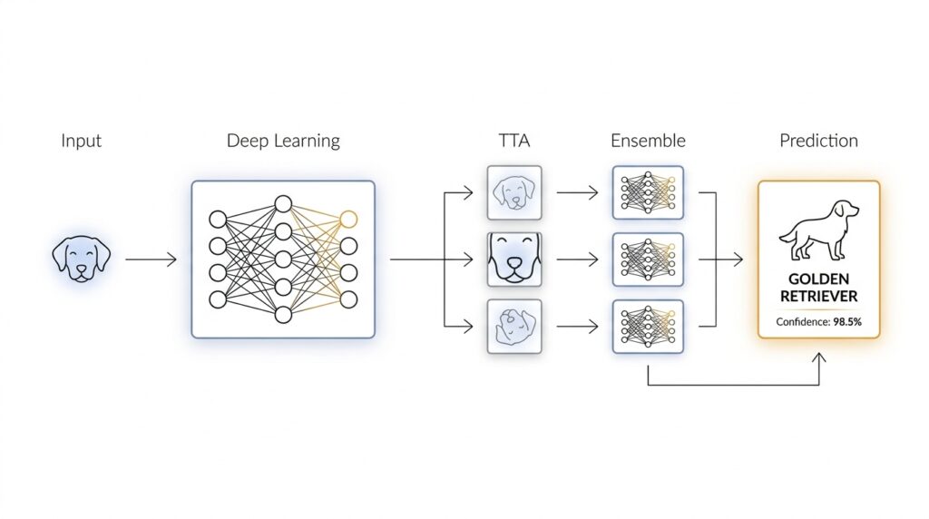
When the fine-tuned dog breed classifier is already making decent predictions, the next question becomes a little more human: what if we gave it a few different chances to look at the same photo? That is the idea behind test-time augmentation, often shortened to TTA. Instead of trusting one single view, we nudge the image in small ways at prediction time, ask the model to respond to each version, and then combine those answers into one steadier result. It feels a bit like asking a friend to identify a dog after seeing it from the front, then from a slight angle, then in softer light.
Test-time augmentation matters because a dog breed classifier can be sensitive to tiny changes in framing. A dog’s ears, muzzle, or coat pattern might sit near the edge of the image, and a single crop can hide the very clue the model needs. If you have ever wondered, “How do I improve dog breed classification without retraining the whole model?” this is one of the first tricks to try. We are not teaching the network a brand-new lesson here; we are helping it make a calmer decision from several closely related views.
The process starts with small, safe transformations. At test time, we might flip the image horizontally, take slightly different crops, or adjust the scale a little so the dog appears in a few nearby positions. These are called augmentations because they create alternate versions of the same input, and they are “test-time” because we use them after training, when the model is already frozen and ready to predict. The key is restraint: we want enough variety to expose the model to different viewpoints, but not so much that we distort the dog into something unfamiliar.
Once those versions are ready, the classifier makes a prediction for each one. In a dog breed classifier, that usually means producing a probability score for every breed, not just a single label. We then average those probability scores, or sometimes take a weighted average, and choose the breed with the highest combined confidence. This is the heart of test-time augmentation: one photo becomes several small opinions, and those opinions blend into a more reliable answer. The model is still the same model; we are simply asking it to look more than once.
What makes this useful is that different crops often reveal different clues. One crop may highlight the face, another may show the coat, and a third may preserve the full body shape. A Basenji and a Shiba Inu, for example, can look surprisingly close in one view and much easier to separate in another. TTA does not fix a weak model, but it can smooth out the model’s uncertainty when the breed is visually ambiguous. In that way, it behaves like a second pair of eyes that notices details the first glance missed.
There is also a practical reason to like test-time augmentation: it often improves predictions without changing training data, loss functions, or architecture. That means we can keep the fine-tuned pretrained model exactly as it is and add a small inference step on top. In machine learning, inference is the stage where the model makes predictions on new data, so TTA lives in the final decision-making moment rather than the learning phase. This makes it a gentle upgrade, which is appealing when we already trust the model and want to polish its output rather than rebuild it.
Of course, TTA asks for a little more computation because the model now processes several versions of each image instead of one. That tradeoff is usually worth it when accuracy matters more than speed, especially in a dog breed classifier where fine visual differences can lead to the wrong answer. The best results often come from a small, deliberate set of augmentations rather than a long, noisy list. With that in place, we have a prediction routine that feels more careful, and that carefulness sets us up nicely for the next step, where multiple models can start working together instead of taking turns alone.
Blend Ensemble Predictions
Once we have a fine-tuned model and test-time augmentation in place, the next challenge is not learning one more trick, but learning how to listen to several good answers at once. That is what blending ensemble predictions means: we take the output from multiple models, or multiple versions of the same model, and combine them into a single final prediction. If you have ever wondered, “How do you combine several dog breed classifier predictions into one answer?”, this is the moment where the puzzle starts to make sense.
The reason blending helps is easy to picture. One model may be especially good at spotting ear shape, another may notice coat texture, and a third may handle unusual lighting better than the others. On its own, each dog breed classifier has blind spots, but together they can cancel out some of each other’s mistakes. Instead of betting everything on one opinion, we let the ensemble of models speak, and then we look for the pattern in their shared confidence.
The most common way to blend ensemble predictions is to average probability scores. A probability score is the model’s confidence for each breed category, and it is more useful than a single label because it shows how strongly the model favors one breed over the others. This is often called soft voting, which means we combine the confidence distributions rather than counting only the final class choice. In practice, this gives us a smoother result than hard voting, where each model casts a single vote and the winning breed takes all.
From there, we can make the blend a little smarter by using weights. A weight is a number that tells us how much influence one model should have compared with another, and it becomes useful when one model consistently performs better on the validation set, which is the held-out data we use to check model quality before the final test. A stronger model might receive a larger weight, while a weaker one contributes a smaller share. That does not mean the weaker model is useless; it simply means we are giving each prediction as much responsibility as it has earned.
This is also where test-time augmentation fits neatly into the story. Each augmented version of an image produces its own set of probability scores, and those scores can be blended within a single model before we blend across models. Think of it like asking one careful observer to look at the dog from a few angles, then asking several observers to compare notes. The final dog breed classifier benefits twice: first from the extra viewpoints inside each model, and then from the broader perspective across the ensemble.
A practical blend usually starts with a small, trusted set of models rather than a huge crowd. Maybe we combine a baseline convolutional neural network, a pretrained model that was fine-tuned on the dog dataset, and another backbone that learned slightly different features. Because each model was trained under different conditions, their errors are often different too, and that diversity is what makes the ensemble useful. If every model makes the same mistake, blending will not rescue us; but if they disagree in healthy ways, the final prediction often becomes more stable.
It also helps to check the blend on the validation set before trusting it on new images. We want to compare not only accuracy, which tells us how often the breed prediction is correct, but also consistency, which tells us whether the ensemble behaves predictably across different kinds of photos. Sometimes a simple average works best because it is robust and easy to reason about. Other times, a weighted blend or a small search over weights gives us a better balance, especially when some models are clearly stronger on certain breeds.
The nice part is that blending does not require us to rebuild the whole pipeline. We keep the individual models intact, gather their prediction probabilities, and combine them at the end like careful editors assembling a final draft. That makes ensemble predictions a low-risk upgrade: we are not changing what each model has learned, only improving how we decide among their answers. And once we have that final, blended score, we are ready to turn a noisy set of guesses into the most reliable breed prediction we can make.
Compare Validation Performance
Now that we have several model variants on the table, the real question becomes which one actually helps our dog breed classifier on unseen images. This is where validation performance matters, because the validation set acts like a rehearsal room: the model does not learn from it, but we use it to see how well the model will likely behave in the real world. If you are wondering, “Which model should I trust when the validation scores are close?”, this is the moment to slow down and compare carefully rather than chase the highest number on a single line.
The first thing we compare is validation accuracy, which tells us how often the model picks the correct breed, and validation loss, which tells us how confidently it is making mistakes. Accuracy is the headline, but loss often gives away the deeper story. A model can reach similar accuracy to another model while still producing less confident, more stable predictions, and that often matters when breeds look alike. In a dog breed classifier, that difference shows up most clearly on tricky classes where one model hesitates less and another swings between breeds.
As we move from the baseline CNN to the fine-tuned pretrained model, we usually expect validation performance to improve in a noticeable way. The baseline gives us a grounded reference point, but the pretrained model often learns richer visual features faster because it already understands general image patterns. That said, better training performance does not automatically mean better validation performance, so we watch for the gap between the two. When training accuracy climbs far ahead of validation accuracy, the model may be memorizing the training set instead of learning breed features that generalize.
Comparing the models side by side also means paying attention to consistency, not just peak scores. One model might finish with the best validation accuracy on a single run, while another model gives more dependable results across multiple folds or training seeds. That matters because deep learning training can be a little noisy, and a one-point difference may disappear the next time we rerun the experiment. So when we compare validation performance, we look for a pattern that repeats, not a lucky spike that shows up once and vanishes later.
Test-time augmentation changes the comparison in an interesting way because it usually improves validation predictions without changing the model itself. Instead of evaluating one image in one form, we evaluate several slightly altered versions and blend the results, which often lowers validation loss and smooths out uncertain predictions. On a dog breed classifier, this helps most when the breed cue is small, off-center, or partially hidden. The important thing to notice is not only whether TTA raises the score, but whether it reduces erratic mistakes on borderline images.
Ensembling adds another layer to the comparison, because now we are not judging a single model in isolation. We are asking whether combining multiple models produces a validation result that is stronger than any one model alone. When an ensemble improves validation performance, it usually means the models are making different mistakes, so their strengths can balance one another. That is why a blended result can feel more trustworthy than a lone winner, especially when two breeds are visually similar and no single model is perfectly certain.
The cleanest way to compare validation performance is to keep the test conditions fair. We use the same validation split, the same evaluation metric, and the same preprocessing so we are comparing model behavior rather than setup differences. Then we look at the full picture: accuracy, loss, stability, and how often each model confuses the same breeds. Once we do that, the decision becomes much clearer, and the best validation performance is usually the one that balances strong scores with steady behavior across the whole dog breed classifier pipeline.