Tokenize and Embed Inputs
Before a language model can think about a sentence, it has to meet that sentence in a form it can handle. That meeting happens in two quiet steps: tokenization and embedding. If you have ever wondered, how does a language model turn raw text into numbers it can work with?, this is the doorway. We take the text apart into manageable pieces, then we give each piece a numerical identity the model can learn from.
Tokenization is the first step, and it works a little like packing a suitcase. Instead of carrying an entire paragraph as one heavy object, we break it into tokens, which are small chunks of text such as words, word pieces, or even punctuation marks. A tokenizer is the tool that makes that split happen. It is designed this way because language is messy: some words are common, some are rare, and some can be built from smaller parts, so tokenization gives the model a flexible way to read almost anything we write.
Once the text is split, the language model still cannot use those tokens directly. Computers do not learn from letters the way we do; they learn from numbers. That is where embeddings come in. An embedding is a learned vector, which means an ordered list of numbers that acts like a coordinate on a map. Each token gets its own vector, and tokens with similar meanings often end up near each other in that space. In other words, embedding turns a token from a label into a place the model can reason about.
This is the heart of the tokenization and embedding pipeline: the tokenizer decides what the pieces are, and the embedding layer decides what those pieces mean to the model. A token like “cat” may become one vector, while a token like “cats” may become another vector that lives nearby if the model has learned that they are related. That numerical structure matters because the rest of the network can now compare, combine, and transform these vectors as it processes the sentence. Without embeddings, the model would see only IDs; with embeddings, it sees patterns.
The process also helps with the practical limits of language models. Since models work with fixed-size vocabularies, tokenization gives them a manageable dictionary instead of an endless list of possible strings. This is why you may see a long word split into smaller subword tokens, or why unfamiliar names can still be represented piece by piece. That flexibility is one reason modern tokenization is so effective: it keeps the language model from getting stuck when the text is new, unusual, or misspelled.
There is another important detail hiding in the background. The embedding layer is not a lookup table frozen in place; it is usually learned during training. As the model studies huge amounts of text, it adjusts the vectors so they become useful for the task of predicting the next token. Over time, the language model learns not only which tokens are common, but also which ones tend to appear in similar contexts. That is what gives embeddings their quiet power: they store meaning in a form the model can actually use.
So when we tokenize and embed inputs, we are not performing a mechanical cleanup step. We are translating human language into the model’s native language. The tokenizer breaks the sentence into pieces, the embedding layer gives those pieces a location in numerical space, and the rest of the model can finally begin its work. If the attention mechanism later feels like a conversation between vectors, that is because this first translation already turned words into something the network can compare, remember, and pass forward.
Implement Self-Attention Layers
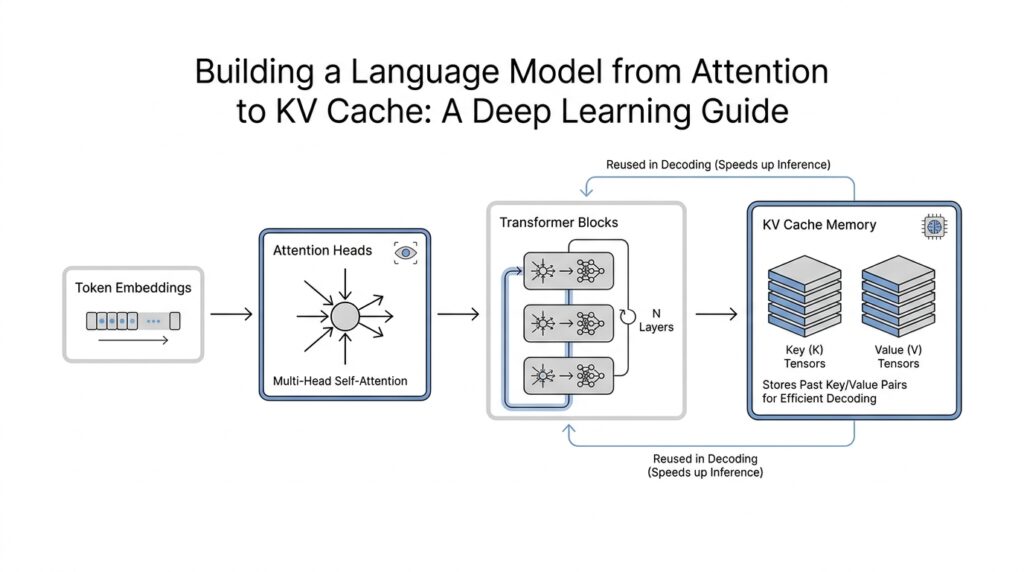
Now that the embeddings are in place, the next question is the one that makes self-attention layers feel magical: how does a language model decide which earlier words matter right now? The answer begins with three learned views of the same input: a query (what this token is looking for), a key (what each token offers as a match), and a value (the information that can be passed along). In the original Transformer, this is the heart of self-attention, where each position can compare itself with the rest of the sequence and build a context-aware representation.
Once we have those three projections, the layer starts a very human-like search. It compares each query against all keys with dot products, scales the scores by the square root of the key dimension, and then runs a softmax, which turns raw scores into a probability-like weight distribution. That scaling step matters because it keeps large dot products from making the softmax too sharp too early. After that, the layer takes a weighted sum of the values, so the token keeps the information that seems most relevant and quietly ignores the rest.
If we are building a language model, though, we have to protect the story’s timeline. A token at position 10 should not peek at token 11 while it is trying to predict the next word, so we add a causal mask—a lower-triangular filter that blocks future positions before the softmax sees them. In PyTorch’s scaled_dot_product_attention, this mask is built by setting illegal future scores to negative infinity, which forces their weights to zero after normalization. That is what preserves the autoregressive behavior that language generation depends on.
Here is where the layer becomes less like a single flashlight and more like a team of explorers. Multi-head attention means we do the same attention process several times in parallel, each time with its own learned projections. The heads are then concatenated and projected again, so one head might focus on nearby grammar while another follows a long-range reference or a repeated phrase. The original paper notes that this helps the model attend to different representation subspaces at different positions, and PyTorch’s nn.MultiheadAttention follows that same design.
When you implement this in practice, the shapes matter as much as the math. PyTorch’s MultiheadAttention layer expects an embed_dim that gets split across num_heads, and when you are doing self-attention, query, key, and value are the same tensor. Under the hood, the module can call optimized scaled_dot_product_attention() when the inputs fit the right pattern, which is one reason modern implementations can run much faster than a hand-rolled loop over tokens. If you have ever searched for “how do I implement self-attention layers in PyTorch?”, this is the path most people eventually take.
The attention output does not usually leave the block alone. In the Transformer architecture, each attention sub-layer sits inside a residual connection, meaning we add the input back to the output before moving on, and then apply layer normalization, which helps keep training stable as signals move through many layers. This matters because self-attention is powerful, but without that little safety rail, the network can become harder to optimize. In a language model, the self-attention layer is not a final answer; it is a well-organized conversation between the token and its context.
So the practical recipe is taking shape: project embeddings into queries, keys, and values; score the matches; mask out forbidden future positions; mix the values; and repeat the whole dance across multiple heads before handing the result to the rest of the block. That is the moment the model stops seeing a sentence as a flat list of numbers and starts seeing it as a living web of relationships. And once we can do that efficiently, we are only one step away from asking how to avoid recomputing the same old keys and values every time we generate the next token.
Stack Decoder Blocks
Once the self-attention layer has given each token a richer view of its neighbors, we reach the next important idea: we do that work again, and then again. What does stacking decoder blocks actually buy us? In the original Transformer, the decoder is a stack of identical layers, and each sublayer sits inside a residual connection followed by layer normalization. PyTorch mirrors that pattern with TransformerDecoder, which is described as a stack of N decoder layers.
Inside each block, the model keeps refining the same sequence rather than starting over from scratch. The decoder’s self-attention sublayer is masked so positions cannot look ahead, which preserves the left-to-right logic needed for language generation, and the block then passes the result through a feed-forward network that transforms each position independently. PyTorch’s TransformerDecoderLayer is built from self-attention, multi-head attention, and a feed-forward network, and it also lets you choose whether layer normalization happens before or after those operations with norm_first.
That repetition is the real reason stacking matters. One block can notice a local pattern, while the next block can build on that updated view and notice a longer dependency, almost like rereading a draft with fresh eyes. The Transformer paper presents this as a simple attention-based architecture that replaces recurrence and convolution, and its base decoder uses six identical layers, which shows that depth was part of the design from the start.
There is also a quiet stability trick hiding in the block. A residual connection means the model adds the input back to the sublayer output, so the original signal stays available instead of getting overwritten at every step; layer normalization then keeps the scale of activations under control. The paper places that residual-plus-normalization pattern around each decoder sublayer, and PyTorch exposes the same choice through norm_first, which is why you will see both pre-norm and post-norm decoder blocks in real code.
If you picture the tensors moving through the network, the flow is easy to imagine: embeddings enter block 1, come out a little more informed, then enter block 2, and so on until the model has built a deep representation of the sequence. The important practical detail is that the stack keeps the feature width, or d_model, fixed across layers, so the sequence can pass through many blocks without losing its shape. That repeated full-stack pass is also why the next optimization question becomes so natural: if every new token has to walk through the same decoder blocks, how do we avoid recomputing work we already did for earlier tokens?
Apply Causal Masking
At this point in the language model, the danger is easy to picture: the model has learned to look around the sentence, but during generation it must not peek at the future. That is where causal masking steps in. In an autoregressive language model, or a model that predicts the next token one step at a time, the mask acts like a row of small curtains that drop over every future position before attention can use it. The Transformer paper describes this as preventing leftward information flow so the decoder preserves its one-token-at-a-time behavior.
How do we stop the model from cheating? We do it right inside the attention scores, before the softmax turns them into weights. In the standard implementation, a causal mask is lower triangular, which means token 5 may attend to tokens 1 through 5, but not to token 6 or beyond. PyTorch’s scaled_dot_product_attention does this with is_causal=True, and its documentation notes that the masked-out positions receive negative infinity so their softmax weight becomes zero.
That detail matters because causal masking is not a separate afterthought; it changes the story the attention layer is allowed to tell. Without it, the model could learn a shortcut by borrowing information from tokens that have not been generated yet, which would make training look better than real decoding. With it, each position only sees the prefix that actually exists, so the model learns the same discipline it will need at inference time. The original Transformer decoder uses this exact rule, and PyTorch’s MultiheadAttention exposes it through the is_causal flag as well.
In practice, the causal mask feels a lot like reading a sentence with a finger under the words. You can move forward, but you cannot jump ahead and spoil the next line. That is why the mask is usually a simple triangle: the shape matches the direction of generation, and the math stays fast because the forbidden scores are removed before the model spends effort normalizing them. PyTorch documents that is_causal applies a lower-triangular mask when the attention matrix is square, which is exactly the case we want for standard decoder self-attention.
There is one practical wrinkle worth noticing when you start writing code. PyTorch treats causal masking in scaled_dot_product_attention as mutually exclusive with a separate attn_mask, so you typically choose one route or the other rather than stacking both. That design keeps the semantics clear: either the function builds the causal barrier for you, or you supply the attention mask yourself. If you are coming from MultiheadAttention, it is worth remembering that the boolean mask conventions differ between these APIs, so the meaning of True is not always the same.
Once the mask is in place, the rest of the attention math can proceed normally. The queries still compare against the keys, the softmax still spreads probability across the allowed past tokens, and the values still carry forward the information that matters most. The only difference is that the model now learns under the same rules it will face when it generates text for real, one token at a time. That is the quiet but crucial job of causal masking in a language model: it keeps the training signal honest, so the decoder can stay faithful to the order of the sentence and prepare us for the next efficiency trick, reusing past attention work instead of rebuilding it from scratch.
Generate Tokens Autoregressively
Now the model has embeddings, masked attention, and stacked decoder blocks, so generation can begin to feel like a rhythm instead of a mystery. We hand the model a prompt, it predicts the next token, and then that new token becomes part of the prompt for the next round. How does a language model write one word at a time without drifting into the future? That is the autoregressive loop: each step depends on the text already produced, not on anything that has not happened yet. The original Transformer was built around this left-to-right decoder behavior, and modern generation APIs still follow the same pattern.
Inside each step, the model emits logits, which are raw scores over the vocabulary before any choice is made. We then turn those scores into a token by taking the highest score, or by sampling from the distribution when we want more variety in the output. This is the part that makes generation feel like a conveyor belt: one prediction is not the end of the story, but the next input to the story. Hugging Face’s generation docs expose this directly, and they describe generated sequences as token-by-token outputs driven by those per-step scores.
The hidden cost appears as soon as the sentence gets longer. Without reuse, every new token would force the model to recompute the keys and values for all earlier tokens in every decoder layer, which means we would keep redoing work that has already been settled. Because causal masking prevents future tokens from changing the past, the model can safely keep those earlier key and value tensors around. Hugging Face’s caching docs spell out the payoff clearly: at inference, we only need the last token’s query, and the new key and value vectors get appended to the stored past. That is why a KV cache turns per-step attention from quadratic work into linear work as the sequence grows.
This is where the KV cache becomes the quiet hero of autoregressive generation. A key-value cache stores the attention keys and values for previous tokens, usually on a per-layer basis, so the model can reuse them during inference instead of rebuilding them from scratch. In practice, the loop becomes very small: process the prompt, keep the cache, feed only the newest token on the next step, and update the attention mask so the model still sees the right prefix length. Caching is for inference, not training, and the cache can grow into a major memory cost for long contexts, which is why modern libraries offer several cache styles for different speed and memory tradeoffs.
Once we see that pattern, autoregressive generation stops looking like a giant leap and starts looking like a careful habit. The model is not trying to invent the whole paragraph in one breath; it is taking one step, checking the context behind it, and then taking the next step with that updated memory. That is why the next-token scores matter so much, and it is also why efficient attention kernels and cache-aware decoding matter so much in real systems. The core idea stays beautifully simple: predict one token, append it, reuse the past, and repeat.
Add KV Cache Support
When a language model starts generating text one token at a time, the first thing we notice is how quickly the same attention work piles up. A KV cache—short for key-value cache—is the trick that keeps that pile from growing into a bottleneck. If you have ever wondered, how do we add KV cache support without changing the model’s behavior?, the answer is to let the model remember the attention keys and values it has already computed, then reuse them during autoregressive generation instead of rebuilding them from scratch.
The easiest way to picture this is to imagine rereading the same pages of a notebook every time you write one new sentence. That would be exhausting. A key-value cache works more like placing sticky tabs on the pages you have already read so you can jump back instantly. During the initial prompt pass, each decoder layer produces its own keys and values for every token, and we store them. On the next step, when only the newest token arrives, the model computes fresh queries for that token and attends against the cached history. That is the heart of KV cache support: preserve the past, update only the present.
In code, this usually means changing the attention layer so it can accept an optional past_key_values input and return an updated cache alongside the attention output. The cache is typically organized per layer, because each decoder block has its own projections and its own attention history. What does a language model need to generate the next token efficiently? It needs the current query, the stored keys and values from earlier tokens, and a clean way to append the new key and value tensors at every step. Once that pattern is in place, the model no longer recomputes attention over the entire prefix each time it takes a new step.
That small interface change has a big effect on performance. Without a KV cache, every new token forces us to revisit all prior tokens in every decoder layer, which makes generation slower as the sequence grows. With caching, the model pays the full cost once for the prompt, then only handles the newest token at each step. This is why KV cache support is so important in real inference code: it turns generation from a repeated full reread into a steady, incremental walk forward. The output stays the same, but the path to get there becomes much lighter.
There are a few details that matter when we wire this up carefully. First, the cache only belongs in inference, not training, because training usually processes complete sequences in parallel and benefits from full attention over the entire context. Second, the cached tensors must stay on the same device and use the same dtype as the model, or memory traffic can erase the speed gains we were hoping for. Third, the attention mask or position logic has to grow with the sequence length so the new token still respects causal masking. If the cache and mask disagree, the model can attend to the wrong positions and produce unstable results.
Support for KV cache also changes how we think about the generation loop itself. Instead of feeding the whole prompt back into every decoder block, we feed the prompt once, save the cache, and then keep passing only the latest token. The cache grows one step at a time, like a ledger that records exactly what the model has already seen. That makes decoding much faster, but it also means memory usage rises with long contexts, so we have to balance speed against storage. In practice, this is the tradeoff that makes KV cache support both powerful and worth handling with care.
Once the cache is in place, the rest of the model feels almost unchanged, which is part of its elegance. The attention math still compares queries, keys, and values; the decoder blocks still stack in the same order; causal masking still protects the timeline. The only difference is that we stop wasting effort on tokens the model already understands. That is the quiet advantage of KV cache support: it keeps the language model faithful to the same generation story we built earlier, while making each new step faster, leaner, and far more practical.