What Are Vector Embeddings?
When we first ask a computer to make sense of language, it feels a little like handing someone a library card and expecting them to read a novel. Words on their own are neat labels, but they are hard for a machine to compare in a meaningful way. That is where vector embeddings step in: they turn a word, sentence, or even a whole document into a list of numbers called a vector (an ordered set of values). In plain language, a vector embedding is a numerical portrait of meaning, which gives vector search something it can actually measure.
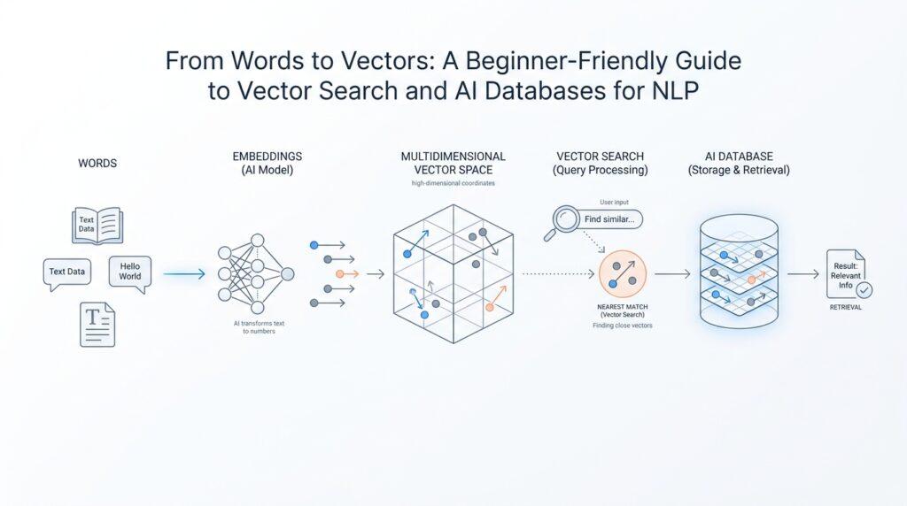
Think about how you might use a map to find a coffee shop. The map does not describe the shop with a poem; it gives you coordinates, and those coordinates make distance visible. Vector embeddings do something similar for language. They place pieces of text into a high-dimensional space, which means a space with many numeric directions instead of the two directions we use on a paper map. The important part is not the exact numbers themselves, but the pattern they create. Texts with related meanings end up near each other, while unrelated texts drift farther apart.
That idea may sound abstract at first, so let’s make it human. If you compare the phrases “cat on the couch” and “dog on the sofa,” a person notices they are closely related even though the words differ. A good embedding model does the same thing by capturing semantic similarity, which means likeness in meaning rather than likeness in spelling. This is why vector embeddings are so useful for natural language processing, or NLP for short, which is the field of teaching computers to work with human language.
Here is the part that makes embeddings feel magical when you see them in action. Two sentences can share almost no words and still land close together in embedding space if they mean similar things. For example, “How do I reset my password?” and “I can’t log into my account” may look different on the surface, but they point to the same user need. Traditional keyword matching might miss that connection, but vector embeddings can catch it because they care about meaning, not just matching letters. That is why vector search can feel smarter than a simple text search box.
Under the hood, an embedding model is the system that creates these vectors from text. You can picture it as a translator that turns language into coordinates a machine can compare. Once the text becomes a vector embedding, the system can measure how close two pieces of text are by using similarity scores, often based on distance (how far apart two vectors are) or cosine similarity (a measure of whether vectors point in the same direction). You do not need the math right away; the key idea is that closeness becomes a stand-in for related meaning.
That is also why embeddings matter so much in an AI database. Instead of storing only words, we store meaning-shaped numbers that can be searched, ranked, and retrieved quickly. This gives us a bridge between messy human language and the structured world a database understands. Once you see vector embeddings this way, they stop feeling like mysterious jargon and start feeling like a practical tool: they are the bridge that lets machines compare ideas, not just strings of text.
How Vector Search Works
Imagine you type a question into a search box and hope it understands the idea behind your words, not just the words themselves. That is where vector search starts its work: it turns your query into an embedding, which is a list of numbers that captures meaning, and then compares that query vector against the vectors already stored in a vector database. The records whose vectors sit closest to your query are treated as the best matches, because embeddings that are near each other usually represent related content.
The easiest way to picture this is to think of a map with many landmarks. Your query becomes one point on the map, and every document, sentence, or product description already lives somewhere else on that same map. Vector search does not ask, “Do these two pieces of text share the exact same words?” It asks, “Are these ideas neighbors?” That is why a search for “I can’t log in” can still find content about password resets, account recovery, or access problems even when the wording is different.
Under the hood, the process has a few steady beats. First, an embedding model converts the query into a vector, and the same kind of vector is stored for each item you want to search. Then the system measures how close those vectors are using a similarity metric, which is a scoring rule that tells us how related two vectors seem; common choices include distance and cosine similarity, which compares whether two vectors point in a similar direction. Smaller distances mean stronger relatedness, so the search engine can rank the closest items first.
If we stopped there, vector search would be accurate but slow on large collections. That is why vector databases usually rely on approximate nearest neighbor search, often shortened to ANN (a fast method that looks for “close enough” matches instead of checking every single vector). Instead of scanning the whole warehouse, the database follows a smart shortcut through the most promising neighborhoods first. Systems like Milvus and Weaviate describe ANN indexes such as HNSW (a graph-based index for fast similarity search) and flat search for smaller datasets, and Pinecone notes that ANN trades a little exactness for much better speed and lower latency.
That speed tradeoff matters because real collections can contain millions of vectors. A brute-force search would compare your query to every stored item, which gets expensive quickly as the dataset grows. ANN keeps vector search practical by narrowing the field before ranking the final candidates, which is a bit like finding the right aisle in a giant library before reading each book spine one by one. In beginner terms, the database is not guessing wildly; it is using an index to focus its effort where likely matches live.
In real applications, vector search often gets one more helper: metadata. Metadata is extra information attached to each vector, such as a category, date, author, or product type, and it lets you narrow the search before the similarity ranking begins. OpenAI’s retrieval tooling also shows how vector search can work alongside keyword search in a hybrid setup, which is useful when you want semantic understanding and exact terms working together. So if you were wondering, “How does vector search work when I need both meaning and a specific word?” the answer is that modern systems can blend both signals instead of forcing you to choose one.
Once you see the flow, vector search feels less mysterious. A query becomes a vector, vectors are compared in a shared space, ANN keeps the search fast, and metadata or keyword signals can refine the results. That is the bridge from raw language to useful retrieval, and it is the reason vector search has become such a powerful tool inside AI databases.
Similarity Metrics Explained
Similarity metrics are the moment vector search stops being abstract and starts becoming practical. Once your query has been turned into a vector, the database needs a scoring rule—a metric, meaning a function that assigns a number to how alike two vectors are—to decide which records rise to the top. That choice matters more than many beginners expect, because the same set of vectors can look close under one metric and surprisingly far under another. In other words, similarity metrics define what “near” means for your data.
Cosine similarity is the metric many people meet first because it cares about direction more than raw size. Picture two arrows pointing the same way: if one is longer but they aim in the same direction, cosine similarity treats them as highly related. Milvus notes that when embeddings are normalized, inner product and cosine similarity become equivalent, and Weaviate says cosine can be implemented by normalizing vectors and using dot product under the hood for efficiency. That is why cosine similarity often feels natural for text embeddings, where meaning matters more than the sheer length of the vector.
Euclidean distance is the straight-line distance between two points, which makes it feel like measuring with a ruler across a map. Here, smaller numbers mean the vectors are closer together, and zero means they are identical. Weaviate documents squared Euclidean distance, which keeps the same ordering while avoiding the square root, and Milvus explains Euclidean distance as the length of the segment connecting two points in n-dimensional space. This metric is helpful when absolute position matters, not just direction.
Dot product sits in a slightly different place. It rewards vectors that point in the same direction and also gives more weight to larger magnitudes, so it behaves a little like measuring both alignment and intensity at once. Milvus describes inner product as useful when you care about magnitude and angle, while Pinecone exposes dotproduct alongside cosine and euclidean as a first-class choice for similarity search. That is also why some systems treat dot product as a similarity score rather than a pure distance metric.
So which similarity metric should you use for vector search? For most text-embedding workflows, cosine similarity is the safest starting point because it matches the idea of “same meaning, different wording” well. If your embeddings were designed so vector length carries useful information, dot product may surface that extra signal. And if your problem is closer to physical space—like coordinates, sensor readings, or other numeric features—Euclidean distance can be the more natural fit. The key lesson is that metric choice is not cosmetic; it changes the story your database tells about relevance.
That is why a good practice is to test a few sample queries and compare the ranking you get under different similarity metrics before you commit. In a small prototype, that might mean checking whether password-reset questions, account-recovery phrases, and billing issues land where you expect. Once you see those patterns side by side, the choice feels less like guesswork and more like tuning a lens, and that lens will shape every result your vector database returns next.
Choosing a Vector Database
By the time you choose a vector database, the question is no longer what a vector is but where those vectors should live. The best choice is the one that matches your search pattern, your filtering needs, and how much infrastructure you want to carry. If your app depends on semantic search, metadata filters, or hybrid retrieval in the same place, those capabilities belong near the top of your checklist.
Which vector database should I choose for a beginner-friendly project? A good first fork in the road is whether you want a managed service or you want to run the system yourself. Weaviate Cloud describes itself as a fully managed vector database in the cloud, and Pinecone documents a serverless architecture that separates read and write paths so each can scale independently. If you want fewer moving parts, managed feels a lot like renting a furnished apartment instead of buying the tools and fixing the plumbing yourself.
Next, look at how the database handles meaning plus exact rules. Real applications rarely search by similarity alone; they also need filters like category, author, product type, or date. Weaviate documents hybrid search that combines vector search with keyword search using BM25, and Pinecone documents metadata filtering on records in the same index. That combination matters because a vector database is most useful when it can answer, find things like this, but only from this slice of my data.
Scale is the other fork in the road. Some systems are built to stay nimble on smaller datasets, while others are tuned for very large collections and the indexing work that comes with them. Milvus documents multiple vector data types and index types for similarity search, and it explains that indexes trade some preprocessing time, space, and RAM for faster retrieval. Weaviate also notes that HNSW indexing scales well to larger datasets and can begin as a flat index before growing into a graph-based one, so the real question is how your vector database behaves as your embeddings pile up.
Finally, test with your own data instead of trusting feature lists alone. A password-reset query, a product question, and a narrow metadata filter can reveal more than a glossy comparison page ever will, because you can see whether the results feel relevant, whether hybrid search helps, and whether the system stays responsive under your workload. That small hands-on trial is where a vector database stops being an abstract category and becomes the tool you would actually want to keep.
Indexing Text for NLP
Before a search system can understand language, it has to give that language a place to live. That is what text indexing does in NLP: it breaks raw text into pieces the machine can store, search, and compare, while leaving room for exact labels and metadata when we need them. In other words, indexing turns a wall of sentences into a structure the search engine can walk through later, which is the quiet setup work that makes vector search and classic text search cooperate instead of compete.
The first move usually happens twice, and that detail matters more than it sounds. At index time, the system analyzes incoming text, and at search time it analyzes the user’s query in a similar way so both sides are converted into compatible tokens, which are small language pieces like words or word fragments. Elasticsearch documents this as using an index analyzer and a search analyzer, and it recommends keeping them aligned so the same idea is represented in the same form on both sides.
Once text has been split into tokens, the search engine can build an inverted index, which is a data structure that maps each token to the documents that contain it. That sounds technical, but the picture is simple: instead of reading every document from start to finish, the engine can jump straight from a word like “password” to the records that mention it. Elastic’s full-text search docs describe this as the backbone of lexical search, and that is why a query can feel fast even across a large collection.
Now comes the part where indexing starts to feel personalized. Different text problems need different analyzers, which are the rule sets that decide how text gets broken apart and normalized; for example, a stop analyzer removes common words like “the,” while an n-gram tokenizer can slice text into overlapping character chunks for partial matching or languages with long compounds. This is the search equivalent of choosing whether we want to keep every pebble on the beach or only the stones that matter for our trail.
It also helps to separate text fields from keyword fields, because they play different roles. A text field is analyzed for full-text search, while a keyword field keeps the original value intact for exact matching, filtering, and sorting. Elastic’s mapping docs show that this choice is made when the index is defined, which is why good text indexing starts with good field design rather than with a clever query after the fact.
For NLP workloads, long documents usually need one more step: chunking, which means splitting a long piece of text into smaller pieces before storing or embedding it. Pinecone documents chunking for long content and recommends keeping chunk IDs and parent-document metadata so you can trace each chunk back to its source, and its metadata filtering lets you narrow retrieval to the right subset before ranking results. That is especially useful when you want a search hit to feel like the right paragraph, not a vague match buried somewhere in a giant file.
This is also where text indexing and semantic retrieval start working side by side. Pinecone and Weaviate both describe hybrid search as a way to combine lexical search, which looks for words and terms, with vector search, which looks for meaning, so a query can succeed even when the wording is slightly off or highly specific. If you have ever wondered, “How do we find the password-reset article when the user only says they cannot log in?” this is the answer: the text index catches the exact clues, and the embedding-based layer catches the intent.
Building a Search Workflow
Now the pieces start moving. A practical vector search workflow begins when you decide what the search should do: find semantically similar content, narrow results with metadata filtering, and fall back on keyword clues when exact wording matters. In a vector database, the query itself becomes a vector embedding, and the system compares it with stored vectors to return the closest matches. How do we build a vector search workflow that feels helpful instead of mechanical? It looks less like one magic box and more like a small relay race, where each stage hands the result to the next.
We start before the search box ever appears. Long documents work better when we split them into chunks, because a search result should point to the right passage, not a giant file with the answer buried somewhere inside; Pinecone recommends chunking long source material and keeping chunk IDs and parent-document metadata so the pieces can be grouped later. This is also the moment to add metadata like category, date, or document type, because those fields become the guardrails that make later filtering useful. Think of it as labeling boxes before a move: the more thoughtfully we label them, the easier the unpacking becomes.
Next, the vectors need a home that can retrieve them quickly. Search systems such as Weaviate and Milvus use vector indexes, often HNSW (Hierarchical Navigable Small World, a graph-based index), to make approximate nearest neighbor search fast enough for large collections; ANN, short for approximate nearest neighbor, means the database looks for close-enough matches instead of comparing every vector one by one. That shortcut is what keeps the vector search workflow responsive as the collection grows, even though it trades a little exactness for speed and lower latency. If you are wondering why vector search feels practical at scale, this is the hidden machinery doing the heavy lifting.
When a user types a query, the same embedding step turns the question into a vector, and then the database searches for nearby results in that shared space. But a good workflow rarely stops there; hybrid search blends vector search with keyword search such as BM25 (Best Match 25), which helps when the user includes an exact product code, medical term, or error message that semantic matching alone might miss. Weaviate runs the two searches in parallel and fuses the scores, and Pinecone supports hybrid patterns that combine dense and sparse signals in a single request. This is where the system stops feeling like a demo and starts feeling like a search product.
After that, metadata filtering trims the search space before or alongside ranking. Pinecone lets you filter records by metadata values, and Weaviate supports filtered vector search so you can combine similarity with structured conditions like category or timestamp. That means the workflow can answer a question like, ‘show me recent billing articles that also feel semantically close to this issue,’ without forcing you to search the entire index. In practice, filtering is the quiet difference between a search result and a useful search result.
Once you see the pieces in order, the workflow becomes easier to reason about: prepare and chunk the text, store vectors with metadata, use ANN-backed indexing for speed, and let hybrid search and filtering shape the final ranking. Elasticsearch’s full-text search docs make the same broader point from the lexical side: exact terms still matter, especially when you need token-level precision alongside meaning. That balance is the real goal here, and it sets us up for tuning relevance with a much clearer picture of how the vector search workflow actually behaves.