Understanding the OVER Clause
When you first meet SQL window functions, the OVER clause is the part that turns a normal calculation into a row-aware one. What does the OVER clause do in SQL window functions? It tells the database how to shape the set of rows a function can see, instead of collapsing everything into one result the way a regular aggregate does. In PostgreSQL’s documentation, a window function call always includes OVER, and that clause determines how rows are split and processed.
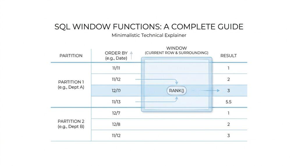
The easiest way to picture it is to imagine a crowd standing in a stadium. PARTITION BY creates the sections of the stadium, and ORDER BY decides how people are lined up inside each section. A partition is a group of rows that share the same values for the chosen columns, while the ORDER BY inside OVER controls the sequence the window function follows for those rows. That order matters even more because it can be different from the order you see in the final query output.
Here is where the idea starts to feel real. Suppose we ask for each department’s salaries, but we also want to know where each employee sits inside that department:
SELECT department,
       employee_name,
       salary,
       row_number() OVER (PARTITION BY department ORDER BY salary DESC) AS salary_rank
FROM employees;
Read that slowly, because the logic is the heart of window functions. row_number() does not count the whole table at once; it counts rows within each department, and the highest salary gets the first number because we told SQL to sort salaries in descending order. That is the practical power of the OVER clause: it lets one query keep every row visible while still performing calculations over a smaller, meaningful slice.
The next piece is the window frame, which is the exact set of rows a function uses at a given moment. This is the part that often surprises beginners, because ORDER BY does not only sort rows; it also changes the default frame for many window calculations. With the default frame, aggregate window functions with ORDER BY often behave like a running total, and functions such as first_value, last_value, and nth_value only look inside that frame rather than the whole partition.
That is why the same OVER clause can feel generous in one query and narrow in another. If you omit ORDER BY, the frame expands to the whole partition, and if you also omit PARTITION BY, the whole table becomes the working set. In other words, OVER is not decoration; it is the instruction manual that tells SQL whether to think in terms of a single group, a sorted group, or a small moving slice inside that group. Once that picture clicks, the rest of SQL window functions becomes much easier to read and predict.
Partitioning Data with PARTITION BY
Picture yourself looking at one big table where sales, salaries, or orders from many groups are mixed together. The question usually arrives the same way: how do we compare each row to the right neighbors without losing the row itself? PARTITION BY is the part of SQL window functions that answers that question by splitting the result set into smaller groups, so each calculation happens inside the right slice of data. In PostgreSQL’s window function model, the OVER clause controls that split, and PARTITION BY divides rows into partitions that share the same values.
The easiest way to think about a partition is as a set of matching name tags. If two rows share the same PARTITION BY value, they belong to the same group, and the window function works on them together; if they do not match, they are kept apart. That is why window functions feel so different from GROUP BY: you still keep every original row in the output, but each row also carries a result that was computed within its own partition. PostgreSQL’s tutorial shows this clearly with row_number(), where each department gets its own sequence and the numbering restarts for the next department.
What if you want each department compared only with itself? That is where PARTITION BY starts to feel natural. Suppose we want the average salary in every department while still listing every employee row, or we want to rank employees within each department without collapsing the table. We can write a query like this:
SELECT depname,
       empno,
       salary,
       avg(salary) OVER (PARTITION BY depname) AS dept_avg,
       row_number() OVER (PARTITION BY depname ORDER BY salary DESC) AS salary_rank
FROM empsalary;
The first window expression gives each employee the average salary for their department, and the second gives each employee a rank inside that same department. The important part is that PARTITION BY depname creates a separate working set for each department, so the average and the ranking never spill across department boundaries. PostgreSQL documents that omitting PARTITION BY creates a single partition containing all rows, which is why the clause matters so much.
PARTITION BY can also use more than one column, and that is where it starts to feel like combining labels on a folder. If you partition by region and product_type, then only rows that match both values land in the same partition. That makes the clause useful when one business idea is not specific enough on its own, such as ranking stores within each region and product line, or comparing monthly revenue inside each country and channel. The database does not treat those columns as separate ideas; it treats them as one combined key for the partition.
It also helps to keep PARTITION BY separate from ORDER BY in your head. PARTITION BY decides who sits in the same room, while ORDER BY decides the order of the chairs inside that room. PostgreSQL notes that the window ORDER BY does not have to match the final output order, and if you omit ORDER BY, the default window frame becomes the whole partition; if you omit PARTITION BY as well, the whole table becomes one partition. That is why a function like sum(salary) OVER (PARTITION BY depname) gives a department total, while adding ORDER BY salary can turn that same idea into a running total inside the partition.
A good reading habit is to translate PARTITION BY into plain language as you scan a query. When you see PARTITION BY depname, read it as “within each department,” and when you see multiple columns, read them as the full rule for who belongs together. That habit keeps window functions from feeling mysterious, because you can tell at a glance whether a calculation is happening across the whole result, inside one partition, or inside a partition that is also ordered. Once that picture is clear, the next step is to see how the ORDER BY and frame details shape the rows inside each partition.
Sorting Rows with ORDER BY
When you add ORDER BY inside OVER, the window function starts reading rows in a specific sequence instead of treating them like a mixed-up pile. That matters because the sort happens inside the window, not necessarily in the final output you see on screen, so the rows can be processed one way while still being displayed another way. If you have been wondering, how do I sort rows inside a window function?, this is the piece that gives the answer.
Think of it like lining up people in a room after we have already decided which room they belong to. PARTITION BY chooses the room, and ORDER BY arranges the chairs inside it. PostgreSQL’s row_number() example shows this clearly: within each department, salaries are ordered from highest to lowest, and tied rows still get numbers, but the order among ties is not guaranteed. In other words, ORDER BY gives the window function its reading order, even when the final query output is arranged differently.
That ordering becomes especially important when we move from ranking to totals. When an aggregate function is used as a window function, PostgreSQL applies it over the current row’s window frame, and with ORDER BY present, the default frame usually runs from the start of the partition through the current row’s last peer. That is why sum(...) OVER (ORDER BY ...) often behaves like a running total instead of a single total for the whole group. The sort order is doing double duty here: it decides sequence, and it quietly shapes the frame the function can see.
Here is a small example that shows the idea in motion:
SELECT department,
       employee_name,
       salary,
       sum(salary) OVER (
           PARTITION BY department
           ORDER BY salary
       ) AS running_department_total
FROM employees;
Read this as a guided walk. First, rows stay inside their own department because of PARTITION BY department. Then, inside each department, PostgreSQL sorts the salaries from low to high. Finally, sum(salary) grows row by row, so each employee sees the total of everyone at or below their place in that sorted sequence. That is the practical heart of ORDER BY in window functions: it turns a flat group into a step-by-step story.
This is also where beginners sometimes feel surprised by functions like last_value(). PostgreSQL notes that first_value, last_value, and nth_value look only at the window frame, not the whole partition, and the default frame with ORDER BY can make last_value() return the current row’s peer instead of the true last row in the partition. If you want the whole partition instead of a moving slice, you can omit ORDER BY or define the frame more explicitly. That small change can completely change the answer, even though the query looks almost the same.
So the safest mental model is this: ORDER BY inside OVER is not the same as the query’s final ORDER BY. It tells window functions how to move through rows inside each partition, like following a trail of footprints rather than reading a shuffled deck. Once you start seeing that distinction, ranking, running totals, and frame-based functions all become easier to predict, because you can ask one simple question: “What order are these rows being seen in?”
Using ROWS and RANGE Frames
Now that we’ve seen how ORDER BY quietly shapes a window, the next question is the one that makes SQL window functions feel precise: how far should the function look? ROWS and RANGE are the two frame modes that answer that question, and the frame is the slice of rows a window function can actually see while it works. In PostgreSQL, a frame belongs to the current partition, and if you do not spell one out, the default is a RANGE frame that starts at the partition beginning and runs through the current row’s last peer.
ROWS is the more literal choice. It counts physical rows in the sorted partition, so ROWS BETWEEN 2 PRECEDING AND CURRENT ROW means “this row and the two rows before it,” like taking three steps back in a line of people. In ROWS mode, CURRENT ROW means the current row itself, and the offset must be a non-null, non-negative integer. That makes ROWS a good fit when you care about position, not about whether nearby rows happen to share the same value.
RANGE works differently, and that difference is the heart of the frame story. Instead of counting rows, it looks at the ordering value itself, so a RANGE frame can include rows whose sort key falls within a value window around the current row. PostgreSQL also requires exactly one ORDER BY column when you use an offset with RANGE, and the offset’s type depends on that column; for numeric sorts, the offset is usually numeric, while for dates and timestamps it is an interval. If you have ever wondered, “Why does my running total include rows that look tied?”, RANGE is often the reason.
That tie behavior matters because RANGE treats peers alike. A peer is a row that matches the current row on the window’s ORDER BY values, and PostgreSQL says the default frame ends at the current row’s last peer, not merely the current row itself. That is why sum(...) OVER (ORDER BY amount) can act like a running total that holds steady across duplicate amounts, while ROWS would advance one row at a time. PostgreSQL also warns that ROWS can be unpredictable if the ORDER BY does not uniquely order the rows, which is another reason to choose the frame mode that matches the question you are asking.
Here is the contrast in a form you can feel. The first window moves by row position, and the second moves by time value:
SELECT order_date,
       amount,
       sum(amount) OVER (
           ORDER BY order_date
           ROWS BETWEEN 2 PRECEDING AND CURRENT ROW
       ) AS last_3_rows,
       sum(amount) OVER (
           ORDER BY order_date
           RANGE BETWEEN INTERVAL '7 days' PRECEDING AND CURRENT ROW
       ) AS last_7_days
FROM sales;
The first column of the frame is like looking at the last three receipts in a stack, while the second is like asking for everything dated within the last week. That difference is exactly what ROWS and RANGE are for in SQL window functions: one follows physical rows, and the other follows values in the sort order.
A useful habit is to choose ROWS when you want a fixed number of sorted rows, and RANGE when you want rows grouped by value distance or tied values to move together. If a result looks surprising, the first thing to check is whether you accidentally left the query on the default RANGE frame, because that default can quietly widen the window to include peers. Once you start reading the frame this way, windowed sums, moving averages, and date-based comparisons become much easier to predict.
Ranking with ROW_NUMBER and RANK
Once we reach ranking in SQL window functions, the story becomes delightfully human: we are no longer asking for totals or averages, but for position. ROW_NUMBER() gives each row a unique place inside its partition, starting at 1, while RANK() gives rows that tie the same position and then leaves gaps after those ties. Both functions need an OVER clause, and both read the rows in the order you define with ORDER BY inside that clause.
That difference matters the moment two rows look equal. Imagine two employees with the same salary: ROW_NUMBER() still hands out different numbers to each row, but the order among those tied rows is not guaranteed unless you add a tiebreaker to the window ORDER BY. RANK(), by contrast, treats tied rows as peers, gives them the same rank, and then skips ahead so the next distinct value lands later in the sequence. In PostgreSQL terms, peers are rows that are not distinct when you look only at the ORDER BY columns.
So which function should you use when two people tie? If you want a clean list with no duplicates in the numbering, ROW_NUMBER() is the right tool. If you want the ranking to reflect the tie itself, RANK() tells the truer story because it preserves the gap between peer groups. A classroom analogy helps here: ROW_NUMBER() is the teacher calling names one by one, while RANK() is the teacher saying, “These two students share third place,” and then moving the next student to fifth place.
A small query shows the difference in action. We can rank employees within each department by salary, and we can see how the two functions react when salaries match:
SELECT department,
       employee_name,
       salary,
       row_number() OVER (
         PARTITION BY department
         ORDER BY salary DESC, employee_name
       ) AS row_num,
       rank() OVER (
         PARTITION BY department
         ORDER BY salary DESC
       ) AS salary_rank
FROM employees;
Here, row_num gives a strict sequence because we added employee_name as a tiebreaker, while salary_rank groups equal salaries together. That is the heart of ranking with SQL window functions: one function gives you a precise row position, and the other gives you a shared place when values tie.
It also helps to read these functions in plain language while you scan a query. ROW_NUMBER() means “the first row, second row, third row, and so on, within this ordered partition,” and RANK() means “the position of this value among its peers, with gaps left behind for ties.” Because the ranking depends on the window order, the final output order can still be different unless you sort the query itself. PostgreSQL’s documentation is very direct about this: the window ORDER BY controls how the function sees rows, not necessarily how the result set is displayed.
That makes these two functions especially useful when you need top-N results, leaderboards, or a reliable way to find “the first few” rows inside each group. ROW_NUMBER() is often the choice when you want exactly one row per slot, even if values tie, while RANK() is better when the business rule says tied values should share the same place. Once you get comfortable with that distinction, SQL ranking functions stop feeling mysterious and start feeling like a clear way to tell a story about order, ties, and importance inside each partition.
Running Totals and Lag Functions
When you first need a running total in SQL, the problem feels simple but a little slippery: you want each row to remember everything that came before it without losing its own place in the story. That is where SQL window functions start to feel especially useful, because they let us keep every row visible while still carrying forward a cumulative sum. If you have ever wondered, how do I calculate a running total in SQL without collapsing the table?, this is the moment where the answer starts to come into focus.
A running total is a sum that grows row by row as SQL moves through an ordered set. In practice, we often write it with sum(...) over (...), and the ORDER BY inside the window is what turns the calculation into a step-by-step climb instead of one flat total. For example, if we sort sales by date, each row can show the amount for that day and the total so far, which feels a lot like adding receipts to a notebook one line at a time. The important idea is that the database is no longer asking, “What is the total for the whole group?” It is asking, “What has happened up to this point?”
That distinction becomes even clearer when we add partitions. If we want a running total per department, per store, or per customer, PARTITION BY keeps each group separate while ORDER BY decides the sequence inside each group. So a sales report can show one cumulative trail for each region without mixing the regions together, which is exactly why SQL window functions are so good at business reporting. The query still returns every original row, but each row now carries a memory of its own partition.
Here is the shape of that idea in code:
SELECT sale_date,
       amount,
       sum(amount) OVER (
         ORDER BY sale_date
       ) AS running_total
FROM sales;
This works because the window reads rows in date order and keeps adding the current amount to everything before it. If you add PARTITION BY customer_id, the total restarts for each customer, which is often what you want when the table holds many independent timelines. The running total is one of those SQL window functions that feels almost like a spreadsheet formula, except it lives inside the database and scales to much larger data.
Once the running total makes sense, LAG() usually appears next as the quiet comparison tool beside it. LAG() is a window function that returns a value from a previous row in the same ordered partition, which means it lets you look backward without writing a self-join. It is especially helpful when you want to compare this row with the one before it, such as checking whether revenue grew, fell, or stayed the same. The function answers a very human question: what changed since last time?
A small example shows the pattern clearly:
SELECT sale_date,
       amount,
       lag(amount) OVER (
         ORDER BY sale_date
       ) AS previous_amount,
       amount - lag(amount) OVER (
         ORDER BY sale_date
       ) AS change_from_previous
FROM sales;
Here, lag(amount) gives the amount from the prior row in date order, and the subtraction shows the difference from one row to the next. On the first row, there is no earlier row to read, so LAG() returns NULL unless you provide a default value. That detail matters, because it reminds us that LAG() is not guessing; it is reaching back only as far as the sorted window allows.
The real power comes when we pair running totals with LAG() in the same query. The running total shows where we are now, while LAG() shows how we got here, which makes the two functions feel like a forward-facing and backward-facing pair of eyes. Together, they can highlight jumps, dips, milestones, and sudden changes in a way that is easy to read in plain language. In SQL window functions, that combination often tells a richer story than either function could tell alone, because one tracks accumulation and the other tracks difference.
A useful habit is to read both functions out loud as you scan the query. sum(amount) over (order by sale_date) means “keep adding as time moves forward,” and lag(amount) over (order by sale_date) means “show me the value from the row just before this one.” Once that rhythm clicks, running totals and lag functions stop feeling like special tricks and start feeling like two very natural ways to follow a sequence of events.