KNN Overview and Intuition
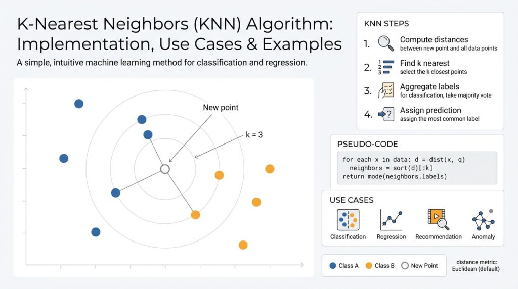
K-Nearest Neighbors (KNN) is one of the simplest yet most instructive machine learning algorithms, and understanding its intuition pays off when you design practical models. At its core, KNN is an instance-based, non-parametric method that predicts a label for a query point by looking at the labels of its closest training examples in feature space. This proximity-driven approach makes KNN conceptually transparent: similar inputs should produce similar outputs, and the algorithm operationalizes that idea using a distance metric and a voting or averaging rule.
The intuition behind “closeness” matters more than the math at first. Imagine each training example as a point in a d-dimensional space; KNN queries that space and returns the k data points whose coordinates minimize a chosen distance function, commonly Euclidean (L2), Manhattan (L1), or cosine similarity for directional data. Because KNN stores examples rather than compressing them into parameters, it adapts naturally to complex decision boundaries where parametric models struggle. This instance-based behavior also means your model capacity scales with data: adding examples refines the local geometry and can reveal new structure without retraining a global model.
Prediction in KNN is operationally simple but flexible. For classification you collect the k nearest neighbors and take a majority vote, possibly weighting votes by inverse distance (e.g., weight = 1 / (distance + eps)); for regression you compute a (weighted) average of neighbor targets. In pseudo-form: neighbors = knn(query, k); prediction = majority_vote(neighbors) or prediction = weighted_mean(neighbors.targets). That direct mapping from neighbors to prediction makes KNN easy to inspect—if you get a surprising prediction, you can look at the contributing neighbors and see why.
Choosing k and the distance metric drives performance trade-offs and requires intentional tuning. Small k (e.g., k=1) fits local idiosyncrasies and tends to low bias but high variance; large k smooths the decision boundary, increasing bias but reducing variance. Feature scaling is critical because distance metrics assume commensurate axes—normalize or standardize continuous features and consider embedding categorical variables with learned encodings. How do you choose k and metric for your dataset? Use cross-validation with stratified folds, evaluate distance metrics on held-out sets, and prefer weighted voting when neighbor distances vary widely.
Practical computation and scalability are common concerns you must address when applying KNN. A naive query costs O(n·d) where n is the number of examples and d is dimensionality; that becomes infeasible for large datasets. For low-to-moderate dimensional data, space-partitioning structures like KD-trees or Ball-trees reduce average-case query time; for high-dimensional or dense embedding spaces, approximate nearest neighbor (ANN) libraries such as FAISS, Annoy, or HNSW trade a bit of accuracy for orders-of-magnitude speedups. Also be mindful of the curse of dimensionality: as d grows, distances concentrate and nearest neighbors become less informative, which is when dimensionality reduction or learned embeddings help.
Real-world use cases illuminate when KNN shines and when it doesn’t. Use KNN as a robust baseline for classification or regression problems, for k-NN imputation of missing values, and for similarity-based tasks like content-based recommendation or image retrieval over vector embeddings—there, cosine or dot-product on learned embeddings often outperforms raw Euclidean distance. Avoid KNN as your primary model for huge tabular datasets with many irrelevant features, or when latency requirements demand guaranteed constant-time predictions without ANN infrastructure. You can, however, combine KNN with other systems: use it for localized corrections on top of a global model or for anomaly scoring by measuring distance to the nearest neighbors.
Building on this foundation, we’ll next implement KNN and explore optimizations like feature preprocessing, metric selection, and ANN indexing so you can apply these intuitions to real datasets. As you proceed, keep the guiding principle in mind: KNN’s power lies in faithful representation of local geometry—design your features and indexing strategy to preserve the neighborhood structure you want the model to exploit.
Distance Metrics Explained
Building on this foundation, the single most consequential design choice you make for KNN is the distance metric: it defines “closeness,” shapes neighborhoods, and directly changes predictions. A distance metric (or similarity measure) formalizes how we compare feature vectors; common choices include Euclidean (L2), Manhattan (L1), and cosine similarity, and each emphasizes different geometric properties of your data. How do you choose the right distance metric for your data? We’ll walk through families of metrics, practical trade-offs, and concrete patterns you can apply when implementing KNN on real datasets.
Start with the Lp (Minkowski) family because it covers the most typical use cases and clarifies behavior. L1 (Manhattan) sums absolute coordinate differences and is robust to sparse, axis-aligned noise; L2 (Euclidean) squares differences so larger coordinate gaps dominate and it favors compact spherical neighborhoods. The Minkowski parameter p interpolates between these behaviors and helps you reason about sensitivity to outliers and feature variance. Remember that a proper metric should satisfy the triangle inequality—this property matters not only mathematically but also for index structures like KD-trees and Ball-trees that rely on metric space properties.
Directional similarity is a different axis of choice: cosine similarity and dot-product measure angle (direction) rather than absolute distance, which is why they shine for embeddings and text representations. When should you prefer cosine over Euclidean? Use cosine when vector magnitude is irrelevant—TF-IDF, sentence embeddings, and many neural embeddings fall into this category—because normalizing vectors before comparison isolates semantic direction. A practical pattern is to L2-normalize your vectors (x := x / ||x||_2) and then use dot(x, y) or cosine(x, y) as your proximity score; this is also efficient in ANN libraries that optimize inner products.
For correlated features or when scale differences persist after preprocessing, Mahalanobis distance offers a principled alternative by incorporating the inverse covariance matrix to whiten feature space. Mahalanobis transforms coordinates so that directions with high covariance are down-weighted, which makes neighborhoods reflect true statistical proximity rather than raw Euclidean gaps. We often use it for anomaly detection or when multiple sensors produce correlated signals; compute S = cov(X) and distance = sqrt((x-y)^T S^{-1} (x-y)). If you need task-specific similarity, consider metric learning (Siamese networks, triplet loss) to learn a projection where Euclidean distance aligns with label similarity.
Real datasets frequently mix numeric, categorical, and ordinal inputs, so naive Euclidean distance on concatenated one-hot vectors can mislead KNN. Use Gower distance for mixed types, or convert categories into dense embeddings learned from the task or via target/mean encoding for high-cardinality variables. Always standardize continuous features (z-score or robust scaling) before distance computations and explicitly weight feature groups when some dimensions are semantically more important; these preprocessing decisions directly change neighborhood topology and therefore KNN performance.
Metric choice also drives computational strategy and evaluation. Space-partitioning indexes assume metric axioms and low-to-moderate dimensionality—if distances concentrate (the curse of dimensionality), nearest neighbors become noisy and ANN methods like HNSW or FAISS with inner-product or cosine support become necessary. Use cross-validation to compare metrics (evaluate weighted voting variants such as 1/(distance + eps)), inspect neighbor distance distributions to detect degeneration, and visualize nearest-neighbor examples when a misprediction occurs. Taking these practical steps ensures your chosen distance metric preserves the neighborhood structure you want KNN to exploit and sets you up to implement efficient indexing and model tuning in the next section.
Feature Scaling and Encoding
Distances drive every KNN decision, so preprocessing that shapes those distances determines whether neighborhoods reflect signal or noise. Building on our discussion of metrics, you must apply feature scaling to numeric inputs and choose encodings for categorical data before you compute proximity—these choices change topology, neighbor order, and ultimately model accuracy. How do you choose scaling and encoding for KNN? We’ll walk through practical patterns, trade-offs, and a reproducible pipeline you can apply to production datasets.
Start with numeric features: scale to make axes commensurate with your chosen metric. If you use Euclidean distance, standardize with z-score (x’ = (x – mu) / sigma) so variance across features is comparable; when outliers dominate a column, prefer robust scaling (median and IQR). For cosine or inner-product similarity, L2-normalize vectors (x := x / ||x||_2) after any centering so direction, not magnitude, drives neighbor ranking. Always fit scalers on training folds to avoid leakage and persist fitted transformers for inference.
Categorical variables require careful encoding because naive one-hot expansion can blow up dimensionality and distort distances. For low-cardinality categories, one-hot or ordinal encoding (when order is meaningful) is fine; for high-cardinality keys, use target/mean encoding with regularization or train small embedding tables to produce dense vectors. When you use target encodings, implement cross-fold or leave-one-out strategies during training to prevent label leakage; when you learn embeddings, treat them like continuous features and scale or normalize them consistently with other inputs.
Combine scaling and encoding inside a deterministic pipeline so KNN sees the same transformations at train and serve time. In scikit-learn terms, compose transformers with ColumnTransformer and Pipeline so numeric columns flow to StandardScaler or RobustScaler and categorical columns flow to OneHotEncoder, TargetEncoder, or a neural embedder. If you weight feature groups (for instance, give text-derived embeddings more influence than raw sensor readings), scale those groups separately and multiply by your chosen weight factor before computing distances so the index and metric reflect your domain priorities.
Practical diagnostics reveal whether preprocessing preserved neighborhood structure: inspect nearest-neighbor examples for a set of queries, plot distance distributions across features, and compute per-feature contribution to L2 distance (delta^2 terms). When dimensionality grows after encoding, watch for distance concentration—if distances collapse, reduce dimensionality with PCA or use learned projections that preserve labels (metric learning). Also consider mixed-type measures like Gower distance when you cannot convert categories without losing interpretability; Gower handles heterogeneous scales while still producing a unified proximity score for KNN.
These preprocessing choices also affect downstream indexing and latency. Space-partitioning trees assume metric properties and low-to-moderate dimensionality, so prefer compact, scaled feature vectors when using KD-trees or Ball-trees; for high-dimensional embeddings, use ANN libraries but keep normalization consistent with the ANN metric (L2 vs. inner-product). By treating scaling and encoding as repeatable engineering steps—validated with cross-validation, neighbor inspection, and leakage checks—you preserve the local geometry KNN depends on and make model behavior predictable as you move toward indexing and production deployment.
Selecting k and Validation
KNN model behavior hinges on a single practical hyperparameter: k. Choosing k correctly and validating that choice determines whether your KNN underfits broad structure or overfits local noise, so you should treat k selection as part of a disciplined validation pipeline rather than a one-off guess. How do you pick k that balances bias and variance while accounting for your distance metric, feature scaling, and class balance? We’ll walk through heuristics, validation strategies, and concrete patterns you can apply in real projects.
Small k (k=1 or 3) gives you razor-sharp local models with low bias and high variance; large k produces smooth, higher-bias boundaries and reduced variance. Start with simple heuristics—try odd k values for classification to avoid ties, consider k ≈ sqrt(n) as a baseline, and test a geometric range (1, 3, 5, 10, 20, 50, …) rather than contiguous integers so you sample both local and global regimes. Also consider weighted voting (weights = 1/(distance + eps)) when neighbor distances vary widely; weighted schemes often let you use a larger k without losing sensitivity to near neighbors.
Cross-validation is the backbone of robust k selection. Use stratified k-fold cross-validation for classification so class proportions are preserved, and prefer 5- or 10-fold splits depending on dataset size; when you’re tuning multiple components (scaling, encoding, metric), use nested cross-validation to avoid optimistic bias in your performance estimate. For time-series or streaming data, replace random folds with time-based splits to respect temporal ordering. Critically, compose preprocessing and KNN inside a pipeline so scalers and encoders are fitted only on the training fold—this prevents leakage and ensures your selected k generalizes.
Pick validation metrics that reflect the task constraints and class balance. For balanced classification tasks, accuracy or F1 can be fine; for imbalanced problems focus on F1, precision-recall AUC, or per-class recall depending on which error mode matters in production. For regression, prefer MAE or RMSE and monitor residual distributions at varying k. Always complement scalar metrics with diagnostic checks: plot neighbor distance distributions, inspect classification boundaries on 2D projections, and sample misclassified queries to examine the contributing neighbors—these qualitative views reveal whether poor performance comes from k choice, feature scaling, or a mismatched distance metric.
A practical tuning workflow embeds KNN inside a reproducible grid or randomized search over k and related choices. Implement a Pipeline that chains ColumnTransformer (scaling and encoding) with the KNeighbors estimator, then run GridSearchCV over n_neighbors, weights (uniform vs distance), and the distance metric when supported. If compute is limited, use a validation holdout for fast iterations and then confirm with full cross-validation; for very large datasets, subsample or use approximate nearest neighbor indexing during tuning to approximate production behavior. Track results with learning curves: plot validation score vs. k and vs. training set size to understand whether adding data or adjusting k is the better lever.
Selecting k and validating it is an interplay between statistics and engineering: you must tune k jointly with preprocessing, metric, and evaluation criterion, and validate under the same constraints your production system will face. In the next section we’ll implement these patterns with pipelines and ANN indexing so you can both find the right k on small experiments and scale that choice reliably to production workloads.
KNN Implementation with scikit-learn
KNN is conceptually simple, but a production-ready implementation requires careful integration of preprocessing, indexing, and validation—scikit-learn gives you the building blocks to do that predictably. In the first 100 words you’ll see the core idea: we compose ColumnTransformer and Pipeline so feature scaling, encoding, and the KNeighbors estimator are trained inside the same cross-validation folds. This ensures no leakage and makes hyperparameter searches reproducible. How do you integrate KNN with preprocessing and hyperparameter tuning in scikit-learn?
Start by creating a deterministic preprocessing pipeline that mirrors the choices we discussed earlier: standardize continuous columns, L2-normalize embedding vectors when using cosine/dot products, and encode or embed categorical features in a way that preserves neighborhood semantics. Use ColumnTransformer to route numeric and categorical columns to the right transformers, then attach KNeighborsClassifier or KNeighborsRegressor as the final estimator. For example:
from sklearn.pipeline import Pipeline
from sklearn.compose import ColumnTransformer
from sklearn.preprocessing import StandardScaler, OneHotEncoder, Normalizer
from sklearn.neighbors import KNeighborsClassifier

preproc = ColumnTransformer([
    ("num", StandardScaler(), numeric_cols),
    ("text_embed", Normalizer(norm="l2"), embed_cols),
    ("cat", OneHotEncoder(handle_unknown="ignore"), cat_cols),
])

pipe = Pipeline([("preproc", preproc), ("knn", KNeighborsClassifier())])
pipe.fit(X_train, y_train)
When you configure the KNeighbors estimator, make explicit choices for n_neighbors, weights, metric, and algorithm because these interact with preprocessing. Prefer odd values of n_neighbors for binary classification to reduce ties, choose weights=”distance” when neighbor distances vary a lot, and select metric=”minkowski” (p=2) or metric=”cosine” after normalizing vectors. For algorithm use “kd_tree” or “ball_tree” on low-to-moderate dimensional numeric data; use “brute” when working with sparse matrices or when you need cosine similarity computed via efficient matrix ops. Also set n_jobs=-1 to parallelize queries during fit/predict.
Tune KNN hyperparameters inside GridSearchCV or RandomizedSearchCV so your preprocessing is refit per fold and your k selection is honest. Nest the pipeline in GridSearchCV and sweep n_neighbors, weights, metric, and leaf_size (which affects tree performance) together. For example:
from sklearn.model_selection import GridSearchCV

param_grid = {
    "knn__n_neighbors": [1, 3, 5, 10, 20],
    "knn__weights": ["uniform", "distance"],
    "knn__metric": ["minkowski", "cosine"],
}
search = GridSearchCV(pipe, param_grid, cv=5, scoring="f1_macro", n_jobs=-1)
search.fit(X_train, y_train)
Once you have a fitted pipeline, use the estimator’s neighbor-inspection APIs to debug predictions—this is one of the strengths of KNN. Call pipeline.named_steps[‘knn’].kneighbors(X_query, n_neighbors=5, return_distance=True) to retrieve the contributing training indices and distances, then inspect those rows to understand failure modes. For classification you can also call predict_proba to see how vote weights translate into confidence; for regression, examine the weighted_mean of neighbor targets and the distribution of distances to detect heteroskedastic regions.
Scalability and deployment matter: scikit-learn’s KNN is excellent for prototyping and medium-scale problems, but for very large datasets or high-dimensional embeddings you’ll likely swap the brute-force search for an ANN index (FAISS, HNSW) in production while preserving your preprocessing pipeline. Persist fitted transformers and any compact index with joblib or the index library’s serialization, and ensure your serving path applies identical normalization/encoding before querying the index. We often use scikit-learn for tuning and sanity checks, then export transformers and embeddings to an ANN-backed serving path to meet latency and throughput requirements.
Building on the validation and metric choices we covered earlier, implement KNN in scikit-learn as an end-to-end pipeline: deterministic preprocessing, scoped hyperparameter search, neighbor inspection for explainability, and a clear migration path to ANN indexing for scale. Next, we’ll explore efficient approximate indexing and how to align ANN metrics with the preprocessing choices you make here so neighborhood structure remains consistent in production.
Speedups: KD-tree and Ball-tree
Building on this foundation, we need indexes that let KNN scale from hundreds to millions of points without paying O(n·d) per query; KD-tree and Ball-tree are two classic space-partitioning approaches that deliver those speedups for many practical datasets. Both trees prune large portions of space during neighbor search so you avoid distance calculations to every example, which dramatically lowers average query time when dimensionality is moderate and preprocessing preserves neighborhood geometry. How do you choose between them for your workload and metric, and when should you fall back to ANN methods instead?
KD-tree partitions space with axis-aligned hyperplanes, so start by thinking in coordinates: we cycle split axes (or choose the largest-variance axis) and place a median cut to create leaf buckets containing small numbers of points. This structure makes KD-tree queries efficient because we can traverse one branch to a leaf then backtrack only into sibling nodes whose bounding hyperrectangles might contain closer neighbors; the pruning relies on the triangle inequality and rectangular bounds, which is why KD-tree shines for low-to-moderate dimensions (roughly up to ~10–30 dims depending on data) and Euclidean-like metrics. In practice you tune the tree by adjusting leaf_size (or leaf_size equivalent in your library) and using axis selection heuristics; these engineering knobs control the trade-off between tree depth, memory, and per-query bookkeeping.
Ball-tree uses hyperspheres (balls) instead of axis-aligned boxes, so its splits create clusters with a centroid and radius that naturally capture non-axis-aligned structure and imbalanced densities. Because Ball-tree bounds are rotationally invariant, it often prunes better than KD-tree when clusters are elongated or oriented diagonally relative to feature axes, and it supports a wider family of metrics directly (including some non-Euclidean distances) because you can define ball coverings in any metric space that respects the triangle inequality. For datasets with correlated features or where meaningful neighborhoods are spherical in the metric you chose, Ball-tree will usually produce tighter node bounds and fewer distance checks than KD-tree, especially when dimensionality is modest but feature orientation matters.
Comparing them in practice: choose KD-tree when your features are well-scaled, roughly axis-aligned after preprocessing, and dimensionality is low; prefer Ball-tree when clusters are rotated, when you need metric flexibility, or when data density varies widely across regions. Remember the curse of dimensionality: both trees degrade as d grows and distances concentrate, at which point approximate nearest neighbor (ANN) libraries (FAISS, HNSW, Annoy) become the pragmatic alternative for high-dimensional embeddings. For example, a 12-dimensional sensor dataset with standard scaling often benefits from KD-tree search, whereas 64–512 dimensional neural embeddings usually require ANN indexes for latency-sensitive production queries.
When you implement these indexes, align tree choice with the preprocessing pipeline we discussed earlier: fit scalers on training folds, L2-normalize if you plan to use cosine-like similarity, and persist the same transformers for serving. Tune parameters such as leaf_size, metric, and algorithm in cross-validation so your index behavior during hyperparameter search matches production. Use KDTree(leaf_size=...) or the Ball-tree equivalent in your toolkit with n_jobs=-1 to parallelize neighbor queries during batch evaluation, and always use the estimator’s kneighbors API to inspect contributing indices and distances when debugging mispredictions.
Beyond parameter tuning, there are practical patterns that improve speed and robustness: build the tree on a dense, compact representation (reduce sparse one-hot expansions with embeddings or PCA before indexing), favor distance-weighted voting when neighbors have widely varying distances, and consider hybrid strategies—use KD-tree or Ball-tree for medium-scale tables and switch to ANN for embedding-heavy retrieval. We’ll take these choices further when we discuss ANN indexing, where we translate the same preprocessing and metric decisions into graph- or product-quantization-based indexes that meet strict latency and throughput constraints.