Define Inventory Intelligence Goals
Building on this foundation, the first thing we want to do is pause before writing more models and ask a quieter, more important question: what decision should this inventory intelligence pipeline help you make? An inventory pipeline can feel productive while still missing the point, because it can produce plenty of counts, trends, and charts without answering whether you should reorder, hold back, discount, or investigate. Think of the goal like the destination on a map—without it, every turn looks reasonable, but none of them prove you’re going the right way.
In a dbt and Python workflow, that clarity matters even more because each tool plays a different role. dbt is built to help you build, document, and collaborate around transformations, while Python models are meant for transformation work that benefits from richer logic such as advanced calculations, text parsing, date handling, forecasting, or feature engineering. That means the goal should tell you where the pipeline needs disciplined SQL-style structure and where it needs Python-driven analysis. If the goal is fuzzy, the architecture becomes fuzzy too, and the inventory intelligence pipeline starts collecting features instead of delivering decisions.
So how do you know what to define first? Start by turning a metric request into a decision question. Instead of saying, “We need inventory turnover,” ask, “What action will we take when a product slows down?” Instead of saying, “We need stockout reporting,” ask, “Which items need attention before demand exceeds supply?” That shift sounds small, but it changes everything. You are no longer building a report that describes the past; you are building a system that helps people act in the present.
Once the decision is clear, the metrics usually fall into place like ingredients in a recipe. If your main worry is stockouts, the core signals might be on-hand inventory, days of supply, lead time, and out-of-stock rate. If your worry is excess inventory, the same inventory intelligence pipeline might lean on sell-through, aging stock, and forecast error. You do not need every possible measure on day one. You need the smallest set of signals that can tell a clean story, because a focused story is easier to trust, easier to test, and easier to improve inside dbt models before you add more sophisticated Python logic later.
It also helps to define the audience behind the goal, because different people need different answers from the same pipeline. A planner may want daily replenishment guidance, a finance partner may care about weekly inventory value, and a category manager may want early warnings for slow-moving stock. When you name the person, the decision, and the timing together, the pipeline becomes practical instead of abstract. You can then decide whether a dbt model should publish a trusted operational metric, whether a Python step should score demand risk, or whether both should feed the same view of truth. That is the real purpose of defining inventory intelligence goals: not to collect more data, but to make the next decision sharper.
As we move forward, this goal-setting work becomes the anchor for every source, transformation, and check we add next. Once we know what success looks like, we can shape the rest of the inventory intelligence pipeline around it with far more confidence.
Ingest Raw Data With Python
Building on this foundation, the next step in an inventory intelligence pipeline is to bring raw data into the room without pretending it is ready to be trusted. This is where Python becomes especially useful, because it can read files, connect to APIs, and shape messy inputs before dbt turns them into reliable models. If you have ever opened a spreadsheet and found duplicate product codes, missing dates, or columns that mean different things in different files, you already understand the problem we are solving. How do you turn that kind of raw inventory data into something the pipeline can actually use?
The first move is to treat ingestion like unpacking boxes after a move. You do not decide where furniture belongs until you know what arrived, what is broken, and what needs to be labeled. In the same way, raw inventory feeds often come from multiple places: warehouse exports, point-of-sale systems, supplier files, or application programming interfaces, which are services that let one system request data from another. Python gives you the flexibility to collect each source, inspect it, and save it in a consistent form before the next layer of the inventory intelligence pipeline takes over.
That flexibility matters because raw data is rarely polite. One file may call the product identifier sku, another may use item_code, and a third may store the same value with leading zeros stripped away. A good ingestion step catches those differences early by standardizing column names, converting dates into one format, and making sure numbers stay numbers. This is not the glamorous part of the work, but it is the part that keeps downstream dbt models from spending their energy correcting avoidable mistakes.
Taking this concept further, think of Python as your first translator. When the source data arrives in different shapes, Python can rename fields, join reference data, remove obvious duplicates, and separate records that failed basic checks. For example, if a supplier file includes both active and discontinued products, you can filter or tag those rows before they ever reach your transformation layer. That means dbt can focus on business logic and modeling, while Python handles the rough edges of ingestion and early cleanup.
Just as important, ingestion should preserve the original truth, not erase it. A strong pipeline keeps a raw landing zone, which is a storage area where incoming data is saved before it is transformed. That way, if a question comes up later about why a stock count changed or why a record disappeared, you can go back and inspect the source exactly as it arrived. This habit makes the inventory intelligence pipeline easier to debug, easier to audit, and much easier to trust when people start using it for decisions.
While we covered goal-setting earlier, now we need to connect those goals to the way data enters the system. If the decision you care about is stockout prevention, your ingestion logic should protect fields like product identifier, location, quantity on hand, and timestamp with extra care. If the decision is about excess inventory, then age, last sale date, and supplier lead time need the same attention. In other words, Python ingestion is not just about moving data around; it is about protecting the signals that matter most to the story you want the pipeline to tell.
Once the raw data is landing cleanly, the rest of the workflow becomes much calmer. dbt can then transform those prepared inputs into standardized tables, test assumptions, and publish models that people can rely on. That is the real handoff we want: Python makes raw inventory data usable, and dbt makes it dependable. From here, we can move from arrival to transformation with far less friction, because the foundation has already been sorted, labeled, and made ready for the next step.
Clean and Enrich Inventory Data
Building on this foundation, cleaning and enriching inventory data is where raw feeds start to feel like one story. How do you turn inventory data that looks almost right into something people can trust? In Python, pandas can convert messy date strings into datetime values, remove duplicate rows, and merge tables with database-style joins, which makes it a strong first stop before dbt takes over.
First, we make the data speak one dialect. That means trimming spaces, standardizing product codes, and converting dates and numbers into consistent types so quantity on hand means the same thing in every file. The tricky part is timestamps: pandas.to_datetime can parse strings into datetime values, and it can also coerce invalid parses to missing values when you want to catch bad rows instead of crashing the pipeline. That gives you a safe place to spot problems before they spread.
Then we deal with duplicates, because inventory feeds often repeat the same SKU, or stock keeping unit, across warehouse exports, point-of-sale files, and supplier extracts. pandas gives you duplicated and drop_duplicates, and the choice of which row to keep becomes a business rule, not an accident. If two rows disagree, you can prefer the newest feed, the most complete record, or the source you trust most. That small decision protects the rest of the inventory intelligence pipeline from phantom stock counts.
Taking this concept further, we start enriching the cleaned inventory data with context. In dbt, a model is a saved transformation step, and dbt’s testing culture is built around checks like unique, not_null, accepted_values, relationships, and freshness. That matters because enrichment is only helpful when the joins stay honest: a product should map to the right lookup table, a location should exist in the right reference data, and stale source data should be visible before a planner makes a decision. dbt’s own docs also frame the workflow around building, testing, running, and version-controlling projects, which is exactly the rhythm you want here.
This is where the story gets practical. You might join inventory records to product hierarchies so a planner can see category and brand, to supplier tables so lead time is visible, and to calendar tables so weekdays, holidays, and fiscal periods are available for analysis. If the feed is time-sensitive, pandas.merge supports database-style joins, and merge_asof can match on nearest keys, which is useful when you need the most recent price, shipment, or count instead of an exact timestamp match. In other words, enrichment turns raw stock levels into a decision-ready picture.
Once the cleanup and enrichment layers are in place, dbt can do what it does best: turn that prepared data into trusted models and test the assumptions behind them. We can check that key fields stay present, that codes stay within expected values, and that upstream relationships still line up after every refresh. This is the quiet payoff of inventory data cleaning: fewer surprises, fewer broken joins, and an inventory intelligence pipeline that tells the same story every time you open it. With that stability in place, we are ready to move from shaping data to measuring it with confidence.
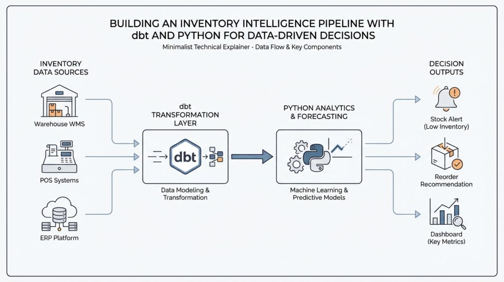
Build dbt Transformation Layers
Now that the raw inventory feeds are landing cleanly, the next question is how we turn them into something people can actually trust and use. This is where dbt transformation layers give the inventory intelligence pipeline its shape: they help us move from messy source records to standardized business logic to decision-ready outputs without letting everything blur together. Think of dbt, or data build tool, as the part of the workshop that turns loose materials into labeled, testable pieces. The layers are what keep that workshop organized.
The first layer is the staging layer, and it should feel close to the source on purpose. In a staging model, we take one raw table and give it a cleaner, steadier voice by renaming columns, casting data types, and standardizing values like location codes or product statuses. We are not trying to make decisions here; we are trying to create a shared vocabulary. If one feed says sku, another says item_code, and a third uses a different date format, staging is where we make those differences disappear before they confuse the rest of the pipeline.
Once the data has a consistent shape, the intermediate layer starts doing the thinking. This is where we combine staged models to express business logic that is useful across multiple reports, such as daily stock snapshots, inventory movement totals, or replenishment signals. If staging is the clean countertop, intermediate models are the prep bowls where ingredients get mixed into something more meaningful. How do you know when to place logic here? A good rule is to ask whether the transformation is reusable and whether it explains how the business works, not just how the source system stores data.
That middle layer is also where the inventory intelligence pipeline becomes easier to reason about. For example, you might calculate days of supply by dividing current on-hand inventory by average daily demand, or you might build a model that flags products with shrinking sell-through and rising age. These calculations often belong here because they support more than one final use case. Instead of repeating the same logic in every report, dbt lets you define it once, test it once, and reuse it wherever the business needs it. That is a small shift with a big payoff: fewer hidden differences and fewer arguments about whose number is correct.
The final layer is where we package the work for real people. These models, often called marts, are the polished tables that planners, analysts, and managers can use without needing to understand the entire transformation chain. A mart might show inventory health by product and warehouse, stockout risk by category, or excess inventory by aging bucket. This layer is where the inventory intelligence pipeline stops being an internal construction site and starts becoming a decision surface. The data should feel familiar here, because it is arranged around the questions people actually ask.
What makes dbt transformation layers so powerful is not only the structure itself, but the discipline around each layer. We can attach tests like unique, not null, and relationships to make sure keys still match, fields still exist, and upstream joins still line up after every refresh. We can also document models so the next person understands why a table exists and what it is supposed to answer. That documentation matters because a pipeline with clear layers is much easier to debug: if a metric looks wrong, we can trace the issue back to staging, intermediate logic, or the final mart instead of searching blindly through everything at once.
As we discussed earlier, the goal is not to create more data for its own sake. The goal is to give the inventory intelligence pipeline a clean path from raw inputs to trusted outputs, and dbt transformation layers are what make that path predictable. When each layer has a single job, the whole system becomes calmer, clearer, and far easier to extend as new inventory questions come up.
Test Data Quality and Freshness
Building on this foundation, the next question is not whether the inventory models look tidy, but whether we can trust them when the business day starts moving fast. A polished dashboard can still hide a missing product code, a broken join, or a source feed that arrived late, and that is exactly where dbt’s data tests earn their keep. In dbt, data tests are assertions about models and other resources such as sources, seeds, and snapshots, and dbt test tells you whether each assertion passes or fails. Out of the box, dbt gives you four generic data tests that cover the most common safety checks: unique, not_null, accepted_values, and relationships.
What makes these tests feel so practical is that they behave like a careful reviewer looking for proof that your claim is wrong. A singular data test is one SQL file that returns failing rows for one specific case, while a generic data test is a reusable parameterized test defined in a test block and then applied wherever you need it. For an inventory pipeline, that might mean writing one-off logic to catch impossible negative on-hand totals in a particular warehouse, while also reusing a generic check that says every product_id should be present wherever inventory rows appear. dbt’s docs emphasize that generic tests are meant to make up most of a test suite because they are reusable and easy to apply across many models and columns.
Once you see it that way, the testing strategy becomes much easier to design. We usually start with the fields that carry the most risk: inventory keys such as product_id, location_id, and supplier_id, plus status fields that drive decisions. A unique test helps ensure one record really means one thing, not_null protects against silent gaps, accepted_values keeps a status field inside the business vocabulary you expect, and relationships checks referential integrity so a row points to a real parent record. In an inventory intelligence pipeline, that matters because a broken lookup can make a stockout look like a normal dip, or make a valid SKU disappear from a report entirely.
While those tests protect the shape of the data, freshness protects its timing. A model can be perfectly structured and still be dangerously old, which is why dbt lets you declare source freshness on incoming tables with a freshness block and a loaded_at_field. You can set warn_after and error_after thresholds so dbt knows when a source is drifting out of date, and then run dbt source freshness to calculate whether each source is fresh enough to trust. Behind the scenes, dbt checks the latest load timestamp, reports pass, warning, or error status, and writes the results to target/sources.json by default.
How do you turn that into a workflow instead of a one-off check? dbt’s recommended pattern is to run dbt source freshness first and then use dbt build --select source_status:fresher+ so only downstream models fed by fresh sources get rebuilt and tested. That is a powerful fit for inventory data, where a warehouse feed might arrive every hour, a supplier file might lag behind, and a finance table might update on a slower cadence. If a source is intentionally infrequent, dbt also allows you to set a table’s freshness to null so you do not keep failing a check that was never meant to be strict in the first place.
The real payoff is that quality and freshness work together like two different kinds of seatbelts. One keeps the data from violating business rules, and the other keeps you from driving with an out-of-date view of reality. When both are in place, the inventory intelligence pipeline becomes much calmer to operate, because every refresh has to prove that the numbers still make sense and that the source data is recent enough to act on. That is the moment where dbt stops feeling like a transformation tool alone and starts feeling like a trust layer for the next decision.
Surface Metrics for Decisions
Building on this foundation, the next job is to turn a pile of trustworthy tables into a smaller set of numbers people can actually act on. This is where the inventory intelligence pipeline stops being a backstage system and starts becoming a decision aid. dbt is designed to transform raw warehouse data into trusted data products, and its Semantic Layer lets us define metrics on top of existing models so the same business number can flow into dashboards, reports, and other tools without being rebuilt each time. That consistency is the difference between seeing data and using it.
How do you know which numbers deserve a place in front of the team? We start by asking what action a metric should trigger, because a metric without an action is only decoration. A primary metric might be stockout risk, while supporting metrics might be days of supply, open purchase orders, and forecast error. Think of the primary metric as the headline and the supporting ones as the paragraph that explains why it matters. In practice, that hierarchy keeps the inventory intelligence pipeline calm enough to read and sharp enough to guide a decision.
Now that the story has a lead character, we need to choose its grain, meaning the level of detail at which the number lives. For inventory, that often means SKU, location, and day, because a warehouse manager and a category manager rarely need the same view. If we surface metrics too broadly, we hide exceptions; if we surface them too narrowly, we create noise. The sweet spot is the smallest level that still matches the decision being made, which is why the inventory intelligence pipeline should publish decision-ready metrics, not every possible slice of the data.
Here is where dbt becomes especially useful: the Semantic Layer centralizes metric definitions in the modeling layer, which keeps different business units from redefining the same number in different places. The docs describe this as moving metric definitions out of the BI layer and into dbt so the same definition is refreshed everywhere it is used. In practice, that means a planner, an analyst, and a finance partner can look at the same inventory intelligence pipeline and see the same meaning behind inventory value or replenishment risk. We are not just publishing data; we are publishing shared language.
Once the metric is defined, we decide how it should reach people. dbt’s Semantic Layer docs describe three useful paths: deploy metrics through a dbt job, query them through downstream tools and applications, and speed common queries with caching or exports. That gives us a practical menu: a daily dashboard for routine review, an alert for urgent exceptions, or an API-backed metric for another system that needs the number in real time. The channel should match the decision speed, because a weekly finance metric and an hourly replenishment metric should not travel the same route.
The last step is to make the surface feel trustworthy. We want each metric to carry a short definition, a clear owner, and a threshold that tells people when to worry, because numbers become useful when they come with context. When you combine that clarity with dbt’s tested models and centralized metric definitions, the inventory intelligence pipeline turns into something people can return to without second-guessing it. From here, we can move into alerting and automation with confidence, because the numbers on the page now mean the same thing to everyone who reads them.