Single-GPU Bottlenecks (docs.pytorch.org)
You can feel a single-GPU bottleneck long before you can name it. The symptoms are familiar: the GPU fans spin, the progress bar moves, and yet the device seems to spend a surprising amount of time waiting instead of working. Why is my single-GPU training still slow? In practice, the answer is rarely one dramatic failure; it is usually a series of small stalls in the training loop, where the CPU prepares data, memory moves across the host-device boundary, and the GPU waits for the next useful task.
The first place we usually look is the input pipeline, because it behaves a lot like a kitchen that cannot keep up with the dining room. PyTorch’s DataLoader is synchronous by default when num_workers=0, which means the main training process handles loading itself and has to wait for data to arrive before it can continue. Turning on worker subprocesses with num_workers > 0 lets data loading overlap with training, and setting pin_memory=True helps the host copy batches to the GPU asynchronously and faster.
Once the data finally reaches the GPU, another kind of single-GPU bottleneck can appear: the work itself may be memory-bound, meaning the GPU spends more time moving values around than performing arithmetic. PyTorch’s tuning guide explains that many pointwise operations, such as elementwise math, are memory-bound and often launch one kernel per operation in eager mode, which adds extra memory traffic and launch overhead. Fusing those operations into a single kernel reduces both memory access and kernel launches, and torch.compile can automate some of that fusion for eligible code.
There is also the quieter problem of launch overhead, which shows up when the training loop keeps asking the CPU to nudge the GPU in tiny increments. Every time the CPU launches a kernel, it pays coordination cost, and the guide notes that CPU-to-GPU work can suffer from extra kernel launches and host synchronization. CUDA graphs are one way to smooth that out, because they keep more of the execution pattern on the GPU and reduce the repeated launch cost that can dominate short or fragmented workloads.
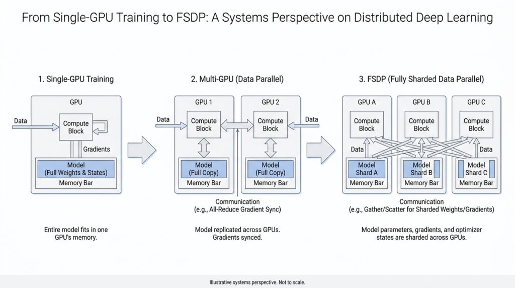
Memory pressure is the bottleneck that often arrives last but feels the most dramatic. A single GPU must hold model parameters, activations, gradients, and optimizer state all at once, so even when compute is available, memory can become the ceiling that stops us from increasing batch size or model size. PyTorch’s checkpointing approach reduces this pressure by storing only some intermediate values and recomputing others during the backward pass, and FSDP goes further by sharding parameters, gradients, and optimizer states so the memory footprint per GPU drops.
Seen this way, a single-GPU bottleneck is less like one broken part and more like a traffic jam with several causes at once. The GPU may be underfed by the data loader, slowed by memory-heavy kernels, interrupted by frequent launches, or boxed in by limited device memory. PyTorch’s distributed tools are designed to reshape those limits: DDP uses multiprocessing to avoid the GIL contention that hurts DataParallel, and FSDP reduces redundancy by sharing the memory burden across devices instead of keeping a full copy on each one.
Data Parallelism with DDP (docs.pytorch.org)
When we move from a single GPU to data parallelism with DDP, the story changes from one worker carrying everything to several workers sharing the same script. Each process holds its own copy of the model, each copy sees a different slice of the data, and DDP keeps those copies aligned by averaging gradients before every optimizer step. PyTorch recommends DDP when your model already fits on one GPU and you want to scale training across more GPUs. What does DDP actually do when the workload gets bigger? It turns multi-GPU training into a synchronized relay instead of a crowd pushing from one doorway.
The first practical step is to launch one process per GPU and create a ProcessGroup, which is the set of workers that agree on how to communicate. Before DistributedDataParallel can wrap your model, torch.distributed must be initialized with init_process_group, and PyTorch notes that nccl is the fastest and most recommended backend for GPUs. This design also gives each process its own Python interpreter, which avoids the interpreter contention that can show up when one process tries to drive many GPUs at once. In other words, DDP does not just spread work around; it also removes a layer of central coordination that can slow the party down.
One detail that surprises beginners is that DDP does not split the input for you. The wrapper synchronizes gradients across replicas, but you still have to arrange the data so that each process gets a different mini-batch, often with DistributedSampler, a helper that assigns non-overlapping pieces of the dataset to each worker. That separation matters because DDP assumes every replica is training on a different slice of the same overall stream, not all chewing on the same batch together. If you are wondering, “Why did my multi-GPU run feel correct but not faster?” this is one of the first places to look.
Under the hood, DDP does a careful bit of bookkeeping before the first backward pass even begins. The constructor broadcasts the model state_dict() from rank 0 so every replica starts from the same weights, then it creates a local Reducer, which is the component that manages gradient synchronization. The Reducer groups gradients into buckets, with bucket size controlled by bucket_cap_mb, and it lays them out in roughly reverse parameter order so the buckets become ready during backpropagation in the order DDP expects. That setup is a little like packing moving boxes in the order you plan to unload them: the details matter because they affect how smoothly the rest of the trip goes.
The real payoff appears during backward. As each gradient becomes ready, autograd hooks mark it for reduction, and when a bucket fills up, DDP launches an asynchronous allreduce, a collective operation that averages values across all processes in the group. Once those reductions finish, the averaged gradients land in param.grad on every rank, so each optimizer step sees the same update everywhere. PyTorch also notes that if you use TorchDynamo, you should wrap the model with DDP before compiling so DDPOptimizer can split the graph around bucket boundaries and overlap communication with compute. That is the quiet superpower of DDP: it keeps the training loop familiar while turning gradient synchronization into a background rhythm instead of a hard stop.
Launching Distributed Jobs (docs.pytorch.org)
Launching distributed jobs is the moment your training script stops being a lone runner and becomes a small team that knows how to work together. With torchrun, PyTorch takes care of the awkward startup details for us: it spawns the worker processes, assigns rank and world_size, and hands each process the environment variables it needs, so we do not have to wire everything together by hand or call mp.spawn ourselves. That is the big shift in distributed training: the launcher becomes the stage manager, and our script can focus on training.
On a single machine, the usual starting point is one process per GPU, because that gives each worker its own slice of work and avoids having one Python process juggle every device. The common launch pattern looks like torchrun --standalone --nnodes=1 --nproc-per-node=$NUM_TRAINERS ..., and --nproc-per-node can even be set to gpu, cpu, or auto depending on the machine. If you have ever wondered, “Why does my multi-GPU job still feel like one process wearing many hats?” this is where the answer begins: each worker must know which GPU it owns, usually through the LOCAL_RANK value that torchrun passes in.
That local rank is the little thread that ties the launcher to the model code. In practice, we read LOCAL_RANK, move the model to that device, and initialize the process group without manually passing rank or world_size, because torchrun has already arranged the coordination for us. PyTorch also notes a small but important compatibility detail: newer launches pass --local-rank, while older scripts may still expect --local_rank, so the argument parser should accept both if we want the same code to survive across versions. This is one of those tiny launch details that feels fussy at first, then saves us from a confusing failure later.
Once we move beyond one machine, the story gains a second moving part: rendezvous, which is the handshake that lets all nodes agree they belong to the same job. For multi-node runs, torchrun asks for a unique --rdzv-id, a --rdzv-backend, and a --rdzv-endpoint, and PyTorch recommends c10d as the default rendezvous backend. The endpoint usually looks like host:port, and the docs warn that if you launch multiple jobs on the same host, each one needs its own port so the jobs do not collide or accidentally merge into one bigger job. That is the distributed launch version of checking that every orchestra reads the same sheet music.
This is also why fault tolerance matters as soon as we care about distributed jobs in the real world. PyTorch’s torchrun tutorial explains that a single process failure can disrupt the whole job, so the launcher can restart workers from the last saved snapshot instead of forcing us to begin from scratch. The snapshot is broader than model weights alone; it can also hold optimizer state, epoch counters, and any other training state we need to resume cleanly. In other words, launching distributed jobs is not only about starting them well, but also about making the restart path feel like part of the plan.
The practical habit is to let the launcher own the fragile coordination pieces and keep our training script boring in the best possible way. We do not hardcode assumptions about stable RANK values or fixed WORLD_SIZE in elastic setups, because those can change after restarts or membership changes. Instead, we write a main() entry point that loads state, initializes distributed communication, and then trains, so the same script can run on one GPU, many GPUs, or many machines with only the launch command changing. Once that layer is in place, we can stop worrying about how the job begins and start paying attention to how the work flows.
FSDP Sharding Basics (docs.pytorch.org)
Now that DDP has given us a steady rhythm, FSDP changes the question from “How do we keep replicas in sync?” to “How do we avoid carrying the whole model everywhere?” The core idea is sharding, which means splitting model parameters, gradients, and optimizer states across ranks so each GPU keeps only a slice when it is idle. Before a layer runs, FSDP gathers the needed pieces back together; after the work is done, it splits them apart again.
That dance feels less mysterious once we follow one layer through the loop. During the forward pass, FSDP all-gathers the parameter shards for that layer, runs the computation, and then frees the full copy again. During the backward pass, it gathers what it needs, computes gradients, and then reduce-scatters those gradients so every rank keeps only its own gradient shard. The PyTorch docs describe this as breaking DDP’s all-reduce into separate all-gather and reduce-scatter steps, which is the key move that makes FSDP memory-efficient.
A useful way to picture this is to think of each GPU as a roommate storing one box of a much larger moving truck. No roommate keeps the entire house in their room, but together they can still rebuild it whenever they need to walk through it. In the same way, FSDP updates sharded optimizer state locally, so the memory savings extend beyond the model weights themselves. That is why FSDP can make models trainable that would otherwise be too large for a single GPU’s memory budget.
FSDP2 makes that picture more concrete with DTensor, short for distributed tensor. After you apply fully_shard, model.parameters() become DTensor objects, and by default FSDP2 shards along dimension 0, so a tensor with N rows spread across N ranks gives each rank one row. One small but important detail follows from that design: you build the optimizer after sharding, so the optimizer sees the distributed parameters rather than an earlier, unsharded copy.
There are also a few sharding strategies, and the names are worth learning because they describe different tradeoffs. FULL_SHARD shards parameters, gradients, and optimizer states. SHARD_GRAD_OP keeps gradients and optimizer states sharded while handling parameters differently around computation. NO_SHARD keeps everything replicated like DDP, while HYBRID_SHARD shards within a node and replicates across nodes to reduce cross-node communication. In the current PyTorch docs, FSDP defaults to FULL_SHARD.
The nice part is that the code stays close to the story we already know from DDP. In FSDP2, you can wrap submodules with fully_shard, and the runtime registers hooks that all-gather before computation and reshard after computation. The tutorial also shows nested wrapping, where inner layers are sharded first and the root model is sharded afterward, which lets FSDP organize communication around the model’s structure instead of treating the whole network as one block.
Once that pattern clicks, FSDP stops feeling like a separate training universe and starts feeling like a thriftier version of the same distributed idea: keep only what you need, only when you need it, and let communication fill in the missing pieces just in time. That is the foundation we need before we look at how FSDP schedules those gathers and scatters so training stays both fast and memory-aware.
Checkpointing Sharded State (docs.pytorch.org)
Once the model is sharded, checkpointing changes from a routine save file into a coordination problem. A state dict is the dictionary of learned weights and other training state, and with FSDP those values may live in pieces across ranks instead of in one tidy block on a single GPU. That is why checkpointing sharded state matters: we want each rank to save the slice it owns, rather than forcing one process to gather the whole model and risk running out of memory. PyTorch’s FSDP docs and distributed checkpointing tutorial both frame this as a normal part of large-scale training, not an afterthought.
The first mental shift is that FSDP can present the same model in different checkpoint shapes. A full state dict gathers everything into one complete copy, while a sharded state dict keeps the pieces distributed, and a local state dict keeps each rank’s local view. For sharded checkpoints, FSDP’s ShardedStateDictConfig lets tensors be saved as ShardedTensor or DTensor, and offload_to_cpu=True can move saved values off the GPU to reduce device memory pressure. In other words, the checkpoint is less like one giant suitcase and more like several labeled carry-ons that stay with the people who packed them.
When it is time to save, the usual move is to tell the root module which state-dict type you want, then call the familiar state_dict() API. FSDP provides set_state_dict_type() and the state_dict_type() context manager for this purpose, and the docs show using StateDictType.SHARDED_STATE_DICT together with the matching optimizer-state config. That matching part matters, because the optimizer state has to follow the same shard layout as the model state; otherwise, loading back later becomes a puzzle with missing pieces. For sharded optimizer state, FSDP’s sharded_optim_state_dict() is the specialized path, and the docs warn that its output is not meant to be fed directly into a regular optimizer loader.
So what happens when we resume? If we stay with the classic FSDP APIs, we load the model weights, transform the optimizer state with optim_state_dict_to_load(), and then hand that result to optim.load_state_dict(). The newer distributed checkpoint APIs make this feel much smoother: get_state_dict() and set_state_dict() can handle FSDP, DDP, tensor parallelism, or combinations of them, and they return keys in canonical FQNs, short for fully qualified names, which are the ordinary module-path names like layer1.weight. The big win is that the saved state can be resharded for a different number of trainers or even different parallelism strategies, which is exactly the kind of flexibility we want when a job restarts in a new shape.
This is also where torch.distributed.checkpoint starts to feel like the friendliest path for real projects. The docs say it writes multiple files per checkpoint, typically at least one per rank, and it uses the storage already allocated by the model instead of trying to build a giant temporary copy first. It also understands stateful objects, meaning it can call state_dict() and load_state_dict() for us when an object follows that protocol, which is why many examples wrap the model and optimizer together in a tiny application-state class. That wrapper turns checkpointing sharded state into a predictable routine: save the shards, keep the names consistent, and let the library do the resharding work on the way back in.
If you are wondering, “How do I checkpoint FSDP without blowing up memory?”, the answer is to keep the checkpoint sharded for as long as possible and only gather what you truly need. Offloading checkpoint tensors to CPU can help, and DCP’s full_state_dict option exists when you really do want one gathered copy, but sharded checkpointing is the more scalable default when the model no longer fits comfortably in one place. That is the quiet promise of FSDP checkpointing: we do not abandon the distributed shape of the model at save time, we preserve it, so the restart path feels like a continuation of training rather than a separate reconstruction project.