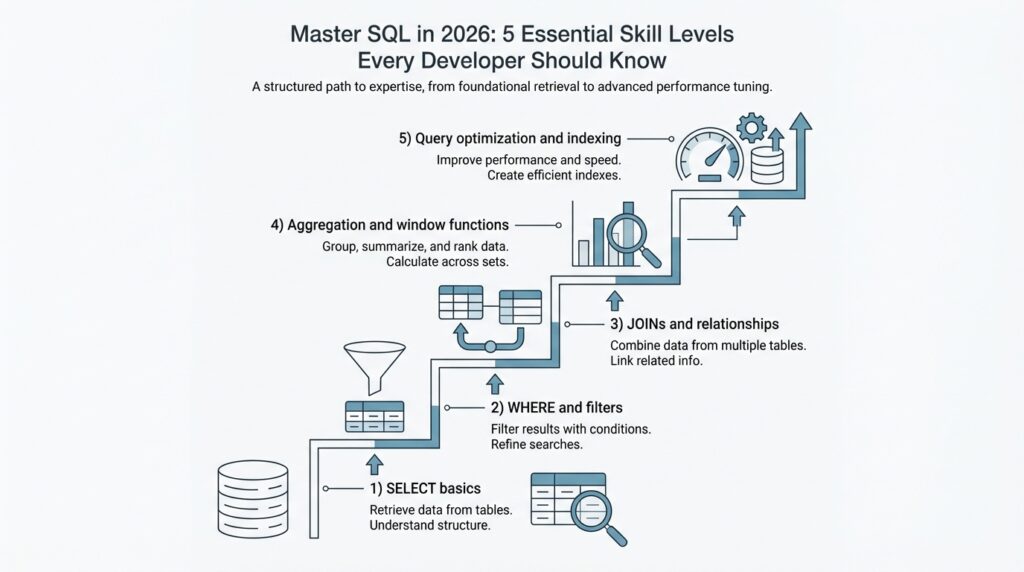
SQL Fundamentals and Data Types
When you first meet SQL, it can feel like opening a filing cabinet and realizing every drawer has a story. A SELECT statement is the part that asks the database for data, and PostgreSQL’s tutorial breaks that request into a select list, a table list, and an optional qualification, which is a helpful way to picture the whole exchange. In plain language, you are saying what you want, where to look, and which rows deserve to come along for the ride. That is the heart of SQL fundamentals: turning a vague question into a clear request the database can answer.
From there, the query starts to feel like a small guided tour. FROM points to the table, WHERE removes rows that do not meet a condition, and ORDER BY arranges the surviving rows in a chosen sequence; if you leave ORDER BY out, the database is free to return rows in whatever order is fastest. When you want a summary instead of a raw list, GROUP BY gathers rows into shared buckets, and HAVING filters those buckets after they form. What is SQL if not a way to ask precise questions in the right order? A query like SELECT city, date FROM weather WHERE city = 'Paris' ORDER BY date DESC; makes that flow easy to see.
Once the query shape makes sense, data types step into the spotlight. A data type tells the database what kind of value a column can hold, and SQL Server groups them into families such as exact numerics, approximate numerics, date and time, and character strings. PostgreSQL’s examples make those families feel concrete: int stores whole numbers, varchar(80) stores variable-length text up to 80 characters, real stores a single-precision floating-point number, and date stores a calendar date. This is why data types matter so much in SQL fundamentals: they are the database’s way of matching each column to the shape of the information it is meant to carry.
The trickier part arrives when values look simple but behave differently. PostgreSQL provides the standard SQL boolean type for true/false values, and it also treats NULL as unknown rather than as a normal value; in SQL’s three-valued logic, true, false, and null do not always act the same inside expressions. That is why a filter can behave differently when a column is missing data, and why WHERE active is not the same mental move as checking for absence with IS NULL. If SQL ever feels fussy here, that fussiness is doing real work for you by keeping truth, falsehood, and uncertainty separate.
So, what data type should you choose for a column? Start with meaning, then narrow it down by range, precision, and how the value will be used later. If it is a count, an exact integer usually fits; if it is text, a character type fits better; if precision matters, exact numerics such as decimal/numeric belong to the safer family, while float and real are the approximate numerics. That habit pays off quickly, because good SQL fundamentals are not about memorizing names—they are about choosing types that help the database understand your data the way you do.
Filtering with WHERE and HAVING
Picture the moment when your query starts to feel crowded. You have rows for every sale, every customer, or every login, and you do not want all of them—you want the rows that earn their place in the answer. That is where WHERE and HAVING step in, and they do very different jobs: WHERE checks individual rows before grouping, while HAVING checks the grouped results after GROUP BY has done its work. In PostgreSQL, the condition in either clause must evaluate to a boolean result, which means it has to come out true or false, not vague or half-finished.
WHERE is the first gate in the story, the one that quietly removes rows before any summary work begins. If we only want paid orders from one country, we use WHERE so the database can throw away the rest before it spends time counting, summing, or averaging anything. That order matters, because PostgreSQL treats WHERE as the stage that decides which rows enter the aggregate calculation at all, and it does not allow aggregate functions there for that reason. So a query like SELECT * FROM orders WHERE status = 'paid'; is not just readable—it is the right place to make a row-by-row decision.
HAVING arrives later, after the rows have already been bundled into groups. An aggregate function is a function like COUNT, SUM, or AVG that compresses many rows into one result, and HAVING is the clause you use when your condition depends on that compressed result. If we group orders by customer and want only customers with at least five purchases, HAVING can inspect the group total and keep or discard the whole group. PostgreSQL also lets HAVING appear without GROUP BY; in that case, the entire result set becomes one group, and the query returns either one row or none depending on whether the condition is true.
The easiest way to remember the difference is to picture WHERE as sorting individual apples before we pack them into boxes, and HAVING as checking the boxes after they are sealed. If the condition does not need a summary—like a date check, a category check, or a status check—WHERE is the better choice because it cuts work early and avoids unnecessary grouping. PostgreSQL’s documentation is explicit about this: WHERE filters input rows before grouping, while HAVING filters group rows after grouping, and a condition that does not involve aggregates is usually more efficiently written in WHERE. That is why WHERE and HAVING are not rivals; they are two filters placed at different points in the same journey.
A practical query makes the pattern click. Imagine we only want customers who have placed at least three paid orders, so we first narrow the raw rows with WHERE status = 'paid', then gather those rows with GROUP BY customer_id, and finally use HAVING COUNT(*) >= 3 to keep only the groups that meet the threshold. The steps read like a small story: choose the rows, build the groups, then judge the groups. Once you feel that sequence in your hands, WHERE and HAVING stop looking like similar filters and start feeling like two precise tools, each waiting for the moment when it can do its best work.
Joins and Relational Thinking
After you’ve learned to filter rows one table at a time, joins are the moment SQL starts to feel social. Instead of treating each table like an isolated notebook page, SQL joins let you place related rows side by side so one table can tell the rest of the story. That is the heart of relational thinking: you look for the relationship between pieces of data, not just the data itself. How do you find the right join when two tables seem to speak different languages? You follow the key that ties them together.
That key is usually a primary key and a foreign key, and this pairing gives the database its map. A primary key uniquely identifies a row, while a foreign key stores a value that must match a row in another table, which is how PostgreSQL describes referential integrity between related tables. Once you see that, joins stop looking mysterious: they become a way of asking, “Which row in this table belongs with which row in that one?” In a well-designed schema, the keys already point the way.
The first join most people meet is the inner join, and it behaves like a careful host who only seats matching pairs. PostgreSQL’s join tutorial explains that an inner join returns rows from both tables only when the join condition matches, while a left outer join keeps every row from the left table and fills in missing right-side values with NULL when no match exists. That difference matters more than it first appears: an inner join answers, “Which records connect?” and a left join answers, “Which records exist even if the other side is missing?” SQL joins become much easier once you hear that distinction in plain language.
The next choice is how you write the join condition, and this is where clarity pays off. PostgreSQL treats ON as the most general form because it accepts a boolean expression, much like WHERE; USING works when both tables share the same column name and removes duplicate output columns; and NATURAL is shorthand for joining on every shared column name, which is convenient but risky if the schema changes later. In other words, relational thinking rewards explicitness. The more clearly you name the relationship, the less chance you have of accidentally joining the wrong pair of rows.
This also explains why some tables come in threes instead of twos. When one order can contain many products, or one student can enroll in many classes, PostgreSQL’s constraint docs show the classic bridge table pattern: a middle table with two foreign keys that connects the two sides and preserves referential integrity. A join through that bridge table feels like walking across two stepping stones instead of trying to leap across a river. Once you recognize that pattern, many-to-many relationships become readable instead of intimidating.
So when you sit down with a schema, start by asking which table owns the identity, which table points to it, and whether a bridge table carries the connection. Then write the join from the key outward, test it with an inner join, and widen to a left join when you want to keep unmatched rows in view. That habit is relational thinking in action: you are not copying data around, you are tracing how the data already fits together.
Grouping, Aggregation, and Reporting
If you have ever stared at a table full of sales, logins, or support tickets and thought, “How do I turn this into something a person can read?”, you have already arrived at grouping and reporting. This is where SQL stops acting like a row collector and starts acting like a storyteller. GROUP BY gathers related rows into buckets, and aggregate functions are the tools that summarize each bucket into one useful number. In SQL reporting, that is the shift that turns a long list into a clear answer.
Think of GROUP BY as sorting mail into labeled trays before anyone counts it. Rows with the same value in a chosen column land together, whether that value is a customer name, a product category, or a month. Once the buckets exist, aggregate functions are the readers who come through afterward and tell us what each bucket contains. COUNT tells us how many rows are there, SUM adds values together, AVG finds the average, and MIN and MAX show the smallest and largest values in the group.
What does GROUP BY do in SQL reporting when the question gets a little more specific? It lets us answer the kinds of questions managers, analysts, and developers actually ask: How many orders came from each city? Which category brought in the most revenue? What was the average response time for each support team? A query like SELECT city, COUNT(*) FROM orders GROUP BY city; does not just return data; it creates a report-shaped summary that is easier to read than the raw table behind it.
The nice part is that grouping and aggregation work best when we keep the result narrow and purposeful. We choose the column that defines the bucket, then we choose the metric that explains the bucket, and we let the database do the counting or adding for us. If we want sales by month, we might group by a month extracted from a date and then sum the amount column. If we want the number of active users per plan, we group by plan and count the rows that belong there. This is the heart of SQL aggregation: one idea for the bucket, one idea for the measurement.
Reporting becomes more powerful when we mix grouped totals with careful filters and readable labels. A report often needs a clean name for each bucket, a sorted order, and a condition that removes noisy groups after the summary is built. That is why GROUP BY and aggregate functions often appear beside HAVING, ORDER BY, and expressions that rename columns into something friendlier for the final output. In practice, SQL reporting is less about pulling data out and more about shaping it into a table that answers a question at a glance.
Once you start thinking this way, you will notice that reporting is really about perspective. The raw rows tell us what happened one record at a time, but grouped results tell us what happened across a crowd of records. That is why aggregation feels so satisfying: it takes the chatter of individual events and turns it into a pattern we can trust. As we move forward, that habit of building summaries will become the bridge to the more polished dashboards and business queries that depend on them.
Window Functions and CTEs
If grouping and aggregation helped us turn a crowded table into a clean summary, window functions are the next small miracle: they let you keep every row visible while still calculating across related rows. That is why people often reach for SQL window functions when they want a running total, a ranking, or a comparison to the previous row without collapsing the result into one line per group. In PostgreSQL, a window function works only with an OVER clause, because that clause tells the database which rows belong to the moving view around the current row.
The easiest way to picture that view is to think of each row standing at a desk with a little frame around it. PARTITION BY splits the data into separate rooms, ORDER BY arranges the rows inside each room, and the window frame decides how much of that room the current row can “see.” That is why the same function can behave differently depending on the setup: a ranking function looks at position, while an aggregate used as a window function can calculate a running sum over the current frame instead of shrinking the whole table into one answer.
This is where window functions start to feel wonderfully practical. row_number, rank, and dense_rank help you see who comes first, who ties, and who shares the same place; lag and lead let you peek at the previous or next row; and ordinary aggregates like SUM or AVG can act as window functions when you add OVER. A question readers often search for is, “How do I calculate a running total in SQL without losing the original rows?” The answer is usually a windowed aggregate, such as SUM(amount) OVER (PARTITION BY customer_id ORDER BY order_date), which preserves each purchase while layering a cumulative total on top.
Once that pattern clicks, CTEs, or common table expressions, arrive like a tidy workbench. A CTE is an auxiliary query inside a larger query, and PostgreSQL treats it like a temporary table that exists only for that statement. That makes CTEs useful when a query starts to feel tangled, because you can give one part of the logic a name, let it do one job, and then use its result in the main query as if you had set the pieces on separate trays first.
That tidy workbench can also change how PostgreSQL plans the work. A non-recursive, side-effect-free CTE may be folded into the parent query, which lets the optimizer treat it more like an inline subquery; if it is referenced more than once, PostgreSQL will normally materialize it, meaning it computes the CTE separately and reuses the result. You can also steer that choice with MATERIALIZED or NOT MATERIALIZED, which is a useful detail when you want to balance repeated computation against index use and query clarity.
There is one more story thread worth knowing: recursive CTEs. When you add RECURSIVE, the CTE can refer to its own output, which is how PostgreSQL handles hierarchical patterns like family trees, category trees, or bill-of-materials structures. That makes CTEs more than a readability trick; they become a way to walk through connected data one step at a time, then hand the finished set to a window function for ranking, labeling, or summarizing.
The real power comes when we combine the two ideas. We might use a CTE to clean and narrow the data first, then apply window functions to rank rows, compare neighbors, or build a running total in the final select. In practice, that pairing gives us a calm, readable query shape: stage the data, name the pieces, and then let the window do its work row by row.
Indexes and Query Performance
The first time a query feels slow, it can seem like the database is being stubborn for no reason. Then we discover indexes, and the whole scene starts to make sense: an index is a separate lookup structure that helps the database find rows without reading the entire table. In PostgreSQL, the default index type is a B-tree, which keeps values in a balanced, searchable order and works well for equality checks and range filters. That is why query performance often changes so dramatically after the right index appears.
A helpful way to picture an index is to imagine the back of a book. Instead of flipping through every page, you scan a short list of topics and jump straight to the right place. A database index works in much the same way, except it points to rows in a table rather than pages in a chapter. When you ask, “Why does one query feel instant while another crawls?” the answer is often that one query can use an index and the other has to search row by row.
But not every index earns its keep. An index helps most when the filtered column is selective, meaning it narrows the search to a small portion of the table. If a query asks for nearly every row, the database may choose a sequential scan, which means reading the table from start to finish, because that can actually be faster than bouncing through an index and then back to the table. We also have to remember the tradeoff: every INSERT, UPDATE, and DELETE must update the index too, so adding too many indexes can slow writes and waste space.
The query planner is the part of PostgreSQL that chooses the route, and it behaves like a careful navigator. It compares the cost of a sequential scan, an index scan, and other paths before deciding what to do, which is why the same SQL query can behave differently as the table grows. This is where EXPLAIN becomes a friend instead of a mystery. It shows the planned execution path, and EXPLAIN ANALYZE shows what actually happened, so you can see whether the database used an index or fell back to a full scan.
Indexes become even more interesting when more than one column matters. A composite index, also called a multicolumn index, stores values from multiple columns together, and the order of those columns matters because PostgreSQL can often use the leftmost part of the index first. That means an index on (status, created_at) may help a query filtering by status and then sorting or narrowing by created_at, while two separate single-column indexes may not be as effective. If a query needs only columns already present in the index, PostgreSQL may even perform an index-only scan, which means it can answer without visiting the table rows themselves.
There are a few common mistakes worth watching for as we build better habits. Wrapping a column in a function, like LOWER(email), can hide it from a normal index unless you create an expression index, which is an index built on an expression instead of a raw column. A leading wildcard in a search like LIKE '%alex' can also make indexing much less useful because the database cannot jump to a clear starting point. The lesson is not to fear SQL indexes, but to match them to the way you actually search, sort, and filter data.
So when a query feels slow, we do not guess blindly; we follow the evidence. We look at the filter, the sort order, the row count, and the execution plan, then we ask whether the table is really being searched in the most efficient way. That habit turns query performance from a vague worry into a practical conversation with the database, and it is one of the clearest signs that you are starting to think like a careful SQL developer.