Think in Sets, Not Rows
When you first approach SQL, it is natural to picture one row at a time, because that is how most programming languages train us to think. But the SQL mental model changes the scene completely: you are not telling the database how to march through records one by one, you are describing the set of rows you want back. What does it mean to think in sets instead of rows? It means you start with the whole shape of the answer and let the database figure out the best path to get there.
That shift matters because a set is more like a basket than a checklist. In a checklist, order and sequence feel important; in a basket, membership is what counts. Modern SQL works best when you imagine collections of data being filtered, combined, grouped, and reshaped as a whole, rather than being processed like a manual loop. This is the heart of set-based thinking, and it is one of the biggest steps from procedural code into the SQL mental model.
Once that idea clicks, clauses like WHERE, JOIN, and GROUP BY start to feel less mysterious. A WHERE clause does not say, “look at row 1, then row 2, then row 3”; it says, “from this set, keep only the members that match.” A JOIN is even more revealing, because it brings two sets together and asks how their rows relate. If you have ever wondered why SQL seems to solve data problems so quickly, the answer is often that it is working on whole sets instead of simulating row-by-row logic.
This is also why beginners sometimes feel surprised by duplicate-looking results. In everyday language, we often expect a table to behave like a tidy list of unique things, but in modern SQL a table can hold repeated values unless you actively prevent them. The database is not judging whether those rows are “the same” in a human sense; it is treating them as members of a result set, and each member matters if it fits the rules you gave. That is a small but important mental turn: the query is about qualifying rows, not narrating a story about individual ones.
Think about it like asking a librarian for every book written by one author, then every borrowed book, then every book that matches both conditions. You would not want the librarian to inspect each shelf in a fixed ritual if they already know how to find the whole answer efficiently. SQL works the same way when you write set-based queries: you describe the destination, and the engine decides how to navigate. That is why the best SQL mental model is less “how do I loop through this?” and more “what collection do I want when the dust settles?”
Aggregation makes this even clearer. When you use COUNT, SUM, or AVG, you are no longer focusing on one row at a time; you are asking the database to collapse a set into a summary. That summary might represent customers, orders, sessions, or events, but the point is always the same: individual rows become members of a larger pattern. If you keep that set-based perspective in mind, GROUP BY stops looking like a strange syntax rule and starts looking like a way to sort a crowd into meaningful buckets.
A helpful question to keep in your pocket is this: am I describing one row, or am I describing the whole result set? That one question can change how you write SQL and how you debug it. When you catch yourself thinking in loops, pause and return to the set-based view, because SQL usually rewards the query that states the desired shape most clearly. Over time, this habit becomes the foundation for writing faster, cleaner, and more reliable modern SQL.
Translate Queries into Algebra
Once you start thinking in sets, the next step is to give those sets a more exact shape. That is where relational algebra enters the picture, because it turns a SQL query into a small chain of operations the database can reason about. If you have ever wondered, “What is the database really doing with my SQL query?”, this is the answer hiding underneath the surface: it is translating your words into relational algebra, then using that structure to plan the work.
Relational algebra is a formal language for describing how tables combine, shrink, and transform. The name sounds intimidating, but the idea is familiar if you picture kitchen prep before a meal. One step washes the vegetables, another chops them, another mixes them, and each step changes the ingredients in a precise way. In the same spirit, a SQL query becomes a sequence of algebraic operations such as filtering rows, choosing columns, joining tables, and grouping results. The point is not to memorize symbols; the point is to see that SQL is a request for transformation, not a script for row-by-row action.
This translation matters because it gives us a cleaner mental model for SQL query structure. A WHERE clause becomes a selection, which means “keep only the rows that match this condition.” A SELECT list becomes a projection, which means “keep only these columns.” A JOIN becomes, at its core, a combination of two relations based on a matching rule. When you translate queries into algebra, you stop seeing clauses as isolated syntax and start seeing them as connected moves in one logical pipeline.
That pipeline also explains why query order in SQL can feel different from the order in which the database reasons about it. We may write SELECT first, but the engine often has to understand FROM, JOIN, and WHERE before it can decide what the final columns should look like. In relational algebra, that makes sense: you cannot project the right columns until you know which rows survive the join and the filter. So when people ask, “How do I translate a SQL query into relational algebra?”, they are really asking how to unwrap the surface syntax into the true shape of the request.
This is where the SQL mental model becomes much sharper. Imagine you are building a result from blocks rather than reciting instructions from a script. Each block in relational algebra has a job, and the database can often rearrange those blocks if the meaning stays the same. That flexibility is one reason modern SQL performs so well: the optimizer can compare different algebraic paths and choose a cheaper one. You do not need to manage that machinery manually, but knowing it exists helps you write queries that are easier to reason about.
You can feel this most clearly with aggregation. A GROUP BY query is not just “count things”; it is a relational algebra step that forms groups and then applies an aggregate like COUNT, SUM, or AVG to each group. That means the database is no longer working with a flat pile of rows but with organized subsets that each produce one summarized answer. Once that clicks, aggregate SQL stops feeling like a special case and starts looking like another transformation in the same algebraic chain.
The practical payoff is confidence. When a query looks confusing, you can slow down and ask what each clause contributes to the algebraic story: which rows survive, which columns remain, which tables are combined, and which groups are formed. That habit keeps you from treating SQL as mysterious magic and helps you read it as a sequence of precise operations. As we move forward, that algebraic way of thinking will keep paying off because it makes deeper query patterns feel like variations on a theme rather than entirely new problems.
Inspect Execution Plans
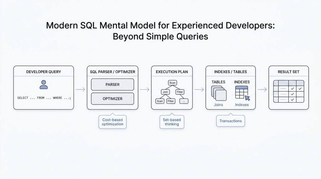
After we can translate a query into relational algebra, the next question gets more practical: what is the database actually planning to do with this SQL? That is where execution plans come in. An execution plan is the optimizer’s chosen route through the data, and official docs across major databases describe it as the plan that shows how rows will be scanned, joined, filtered, and returned. In other words, the SQL query plan is the story behind the result, and reading that story is one of the fastest ways to understand why a query feels brisk or painfully slow.
The first thing to notice is that a plan is not a mysterious wall of jargon; it is a sequence of physical choices. PostgreSQL’s documentation, for example, says the plan shows whether tables are read by sequential scan or index scan and which join algorithms are used to combine inputs, while MySQL’s EXPLAIN reports how tables are joined and in what order. That means the database is taking your logical request and turning it into a concrete workflow, like choosing the shortest path through a warehouse rather than walking aisle by aisle in the order you happened to ask the question.
So how do you inspect execution plans in practice? Most engines give you a way to ask. PostgreSQL uses EXPLAIN, and EXPLAIN ANALYZE goes one step further by actually running the query and showing real row counts and runtime information for each plan node; MySQL uses EXPLAIN to display the optimizer’s view of the statement; and SQL Server exposes estimated and actual plan tools through its query processing and profiling features. The names differ, but the habit is the same: you ask the engine to show its reasoning before you assume the SQL text tells the whole performance story.
Once you have a plan on screen, the most useful comparison is usually between estimated and actual. Estimated numbers come from the optimizer’s prediction, while actual numbers come from executing the query and measuring what really happened. PostgreSQL notes that EXPLAIN ANALYZE adds profiling overhead and that the planning time is separate from execution time, which is a helpful reminder that the plan itself is part of the work too. When those estimates and actual results diverge, you have found a clue, not a failure: the database may have guessed wrong about row counts, data distribution, or the best join strategy.
This is why row estimates matter so much. A plan can look reasonable on paper and still lead the optimizer down the wrong corridor if it expects 10 rows but meets 10 million. The result is often a different scan type, a different join method, or a much larger sort or hash step than you expected. If you are wondering, “Why is my SQL query slow even though it looks clean?”, execution plans are often where the answer waits, because the problem is usually not the syntax but the shape of the work the optimizer believes it must do.
A good reading habit is to follow the plan from the bottom up and ask simple questions at each step. Which table starts the work? Which filter removes rows early? Which join combines the biggest sets? Which operator looks expensive because it must sort, hash, or scan far more data than expected? PostgreSQL even warns that plan reading takes practice, and that is reassuring rather than discouraging: we are learning to read a new kind of map, not memorizing a single fixed answer.
That is the real payoff of inspecting execution plans. Instead of treating SQL as a black box, you begin to see how the optimizer turns set-based intent into physical steps, and you can connect those steps back to the relational algebra we already built. Over time, execution plans stop feeling like after-the-fact debugging output and start feeling like a conversation with the database about how it thinks.
Use CTEs for Clarity
Once you can read execution plans, the next question becomes more human: how do you make the query itself easier to follow? A common table expression, or CTE, gives you that breathing room. It is a named subquery, which means you can break a long SQL statement into smaller labeled steps instead of asking your reader to decode one giant block at a time. In practice, that turns a tangled query into something closer to a guided walk.
Think of a CTE like setting out mixing bowls before you cook. Each bowl holds one intermediate result, and each label tells you what role it plays in the final dish. The database documentation describes a CTE as a temporary result set that lives only for the scope of a single statement, and that same statement can reference the name later on. That matters because the name becomes a signpost: instead of rereading a nested subquery, you can see what the query is trying to do at each stage.
This is where CTEs shine for readability. If you have a query that filters raw events, joins customer data, and then aggregates the result, you do not need to force all three ideas into one sentence. You can name the first step filtered_events, the second event_customers, and the third daily_totals, then read the final SELECT as the last step in a small story. That kind of structure fits the set-based mental model we already built, because each CTE names one intermediate set instead of hiding it inside parentheses.
If you have ever searched for “how do I make a long SQL query easier to read?”, this is the pattern you are probably looking for. The trick is to let each CTE answer one question and one question only: which rows belong here, which rows get enriched here, and which rows get summarized here. That separation does more than tidy up syntax. It gives you checkpoints, so when a result looks wrong, you can inspect the query one stage at a time instead of hunting through a wall of nested logic.
A CTE also helps us keep our expectations honest. It is a writing tool first, not a magic spell that forces the database to execute each block in the exact way we imagine. The optimizer still gets to choose how to run the statement, and MySQL’s documentation explicitly points readers to CTE optimization through merging or materialization. So the real win is clarity: we make the logic easy for people to read, and we let the engine decide the best physical path underneath.
There is one more quiet advantage worth keeping in mind. CTEs can reference earlier CTEs in the same statement, and recursive CTEs can even reference themselves when you need to walk a hierarchy or generate a sequence. That means the same naming pattern that helps with a simple report can also scale into more advanced work later on. For now, the habit to build is straightforward: name intermediate sets after their meaning, keep each step focused, and let the final SELECT read like the last, clean sentence in the story.
Apply Window Functions
After we’ve learned to shape data as a set, the next surprise is that SQL can also keep each row in view while still computing something bigger around it. That is the promise of SQL window functions: they let you look at a row in context, as if you were standing beside its neighbors instead of flattening the whole crowd into one summary. If you have ever wondered, “How do I calculate a running total without losing the original rows?”, this is the pattern you were looking for.
The easiest way to feel the difference is to compare a regular aggregate with a window function. An aggregate like SUM(amount) collapses rows into one answer per group, while a window function like SUM(amount) OVER (...) keeps every row and adds a calculated column beside it. That means you can show each order, each event, or each payment and still attach group-level insight right next to it. In SQL window functions, the row does not disappear; it becomes part of a moving frame of reference.
The OVER clause is the doorway into that frame. Inside it, PARTITION BY means “split the result into separate mini-baskets,” usually by customer, account, or day, and ORDER BY means “put the rows in a meaningful sequence inside each basket.” Once you read it that way, the syntax feels less like a trick and more like a sentence: “For each customer, in date order, show me the running total.” That is why SQL window functions feel so useful in reporting queries, dashboards, and analytics work where the original row-level detail still matters.
Here is a small example of the idea in motion:
SELECT
  order_id,
  customer_id,
  order_date,
  amount,
  SUM(amount) OVER (
    PARTITION BY customer_id
    ORDER BY order_date
  ) AS running_total
FROM orders;
This query does not replace each customer’s orders with one total. Instead, it adds a running_total column that grows as you move through time for each customer. That is the mental shift: we are no longer asking for one answer per group, but for one answer per row, informed by the group around it. In practice, window functions let you layer analysis onto a result without throwing away the detail that made the result interesting in the first place.
The next piece of the puzzle is the window frame, which is the exact slice of rows used for the calculation. Think of PARTITION BY as choosing the room, ORDER BY as arranging the chairs, and the frame as choosing which chairs are included for this specific moment. By default, many database engines use a frame that changes with the current row, which is great for running totals but can be confusing when you expect a fixed range. This is one of the places where SQL window functions reward careful reading, because a tiny change in frame rules can change the answer in a very real way.
Window functions also shine when you need comparison instead of accumulation. Functions like ROW_NUMBER(), RANK(), LAG(), and LEAD() help you ask questions such as “Which row came first?”, “What is the next value?”, or “How does this row compare to the previous one?” ROW_NUMBER() gives each row a position, RANK() handles ties in a more human way, LAG() looks backward, and LEAD() looks forward. Once you start using these tools, SQL window functions stop feeling like a niche feature and start feeling like a conversation with time, sequence, and relative position.
A helpful way to choose between aggregation and windowing is to ask what you want to preserve. If you want one row per customer, use grouping. If you want every order plus the customer’s total, average, or rank beside it, use a window function. That question keeps the design clear: do we want to compress the set, or do we want to annotate it? The answer usually tells you whether a regular aggregate or SQL window functions belong in the query.
This also fits neatly with the earlier habit of breaking work into named steps. A CTE can prepare the rows, and a window function can enrich them without forcing you to repeat logic or nest everything inside one dense expression. That combination often reads like a story: first we find the relevant rows, then we order them, and then we attach the insight that only appears when each row can see its neighbors. Once that rhythm feels natural, window functions become one of the most elegant tools in the SQL mental model.
Tune Indexes and Transactions
After we’ve learned to read execution plans, we usually discover that the next big gains live in two quieter places: index tuning and transaction management. An index is a separate data structure that helps the database find rows faster, and a transaction is a bundle of changes the database treats as one unit so they either all succeed or all fail together. If a query still feels slow after the SQL itself looks clean, this is often where we start looking, because the optimizer can only be as smart as the access paths and concurrency rules we give it.
The easiest way to think about SQL index tuning is to imagine giving the database a better map, not a louder command. PostgreSQL says indexes help queries with WHERE and JOIN conditions, and it will use an index when it thinks that is cheaper than a sequential table scan; MySQL says the same basic thing and adds an important warning: unnecessary indexes waste space and slow down inserts, updates, and deletes because each index must be maintained. That trade-off is the heart of index tuning. We are not trying to index everything; we are trying to index the columns that matter most to the real workload.
That is why a good index is usually shaped around the query pattern, not around a single column in isolation. When one index can support the columns you filter, join, or sort on repeatedly, the database has a better chance of using it efficiently, and PostgreSQL’s own examples show plans shifting from a sequential scan to an index scan or even an index-only scan. An index-only scan is a special case where the database can answer the query from the index alone, without visiting the table data, but only when every column needed by the query is already stored in the index. So when we ask, “How do I tune SQL indexes without hurting writes?”, the answer is usually: build fewer indexes, make them more intentional, and verify that the plan actually changes.
Transactions ask a different question, but the same mindset applies: how long are we holding the door open while other work is trying to pass through? MySQL’s documentation warns that long-running transactions preserve old row versions, delay purge work, and can even prevent other queries from using covering index techniques on those rows. PostgreSQL makes a related point from the isolation side: READ COMMITTED shows each statement the data committed before that statement began, while higher isolation levels provide a more stable snapshot and may require retries when concurrent updates collide. In practice, that means transaction management is not only about correctness; it is also about how long we keep locks, row versions, and concurrency pressure alive.
That is where the tuning habit becomes wonderfully concrete. If a transaction only needs to read a little data, keep it short and choose the weakest isolation level that still protects the business rule you care about. If it needs to write, do the minimum work inside the transaction and commit as soon as the unit of work is complete, because longer transactions widen the window for contention and stale snapshots. MySQL describes isolation levels as a balance between performance, consistency, and reproducibility, and PostgreSQL notes that some update-heavy repeatable-read transactions must be retried when concurrent changes win the race. We are not trying to eliminate concurrency; we are trying to make it behave predictably.
So the practical rhythm is simple: use EXPLAIN to see whether the planner is choosing a scan you expected, add or reshape indexes only when the workload proves they help, and keep transactions as brief as your correctness rules allow. The database is happiest when index tuning and transaction management work together: one reduces the amount of data we must touch, and the other reduces the time we spend holding that data open. Once you start asking both questions every time a query feels slow, you begin to see performance less as a mystery and more as a conversation with the engine.